Reinforcement Learning for Football Player Training
As the most popular sport on the planet, millions of fans enjoy watching Sergio Agüero, Raheem Sterling, and Kevin de Bruyne on the field. Football video games are less lively, but still immensely popular, and we wonder if AI agents would be able to play those properly. Researchers want to explore AI agents’ ability to play in complex settings like football. The sport requires a balance of short-term control, learned concepts such as passing, and high-level strategy, which can be difficult to teach agents. We apply RL to train the agents to see if we can achieve good performances.
- Introduction
- Environment
- Algorithm
- Experiment Results
- 🚀 Extend to real world football matches
- Hyperparameters
- Conclusion and Future work
- Hardware
- Reference
Introduction
In this work, we will utilize the football simulation platform provided by Google Research. The goal is to train an intelligent agent to play football that can achieve the highest score. More detailed information can be found in Google Research Football with Manchester City F.C.
The primary goal of this project is to explore the SOTA methods used in RL to see how well they work in football tactics. We will also try to reproudce the results in paper[1]. In the end, we will show how we can extend our algorithms to real world football matches.
Environment
The environment we are using is Google Research Football Environment. The advantage of the environment is that it’s a widely used football simulator. For example, there is a kaggle competition hosted before where this environment is extensively used. This guarantees that we won’t encounter any unexpected problems while developing our algorithms.
Here are some video demos for the environment integrated with OpenAI Gym.
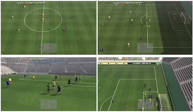
The complete Google Research Football environment can render more realistic graphics and let human players to take over the match.
Here are some screenshots of the environments.
 The following is a video demo of the environment.
Observations & Actions
The environment exposes lots of useful information about two teams, here are some examples of the observations:
Ball Information
- ball [x, y, z] position of the ball
- ball_owned_team {-1, 0, 1}, -1 = ball not owned, 0 = left team, 1 = right team
- ball_owned_player {0..N-1} integer denoting index of the player owning the ball
Left Team
- left_team N-elements vector with [x,y] positions of players
- left_team_direction N-elements vector with [x, y] movement vectors of players
- left_team_yellow_card N-elements vector of integers denoting number of yellow cards a given player has (0 or 1)
Match state
- score pair of integers denoting number of goals for left and right teams, respectively.
- game_mode current game mode, one of:
- 0 normal mode
- 1 kick off
- 2 goal kick
- 3 free kick
Multi-Agent Support
The default mode of the environment is that only one single player is controlled when playing the game. However the environment does support multiple agents. We just need to specify which players to control like the following
python3 -m gfootball.play_game --players=gamepad:left_players=1;lazy:left_players=2;bot:right_players=1;bot:right_players=1;bot:right_players=1
In this work, we will focus on single player mode and leave the work on multi-agents to future work.
Scenarios
GRF(Google Research Football) comes with a lot of scenerios that are common in real football matches such as 11_vs_11, academy_run_to_score, academy_3_vs_1_with_keeper, etc. We will only work on a few representative ones in our work and leave the rest to future work.
Algorithm
The 3 algorithm we explored in our work are: DQN, PPO, IMPALA.
DQN
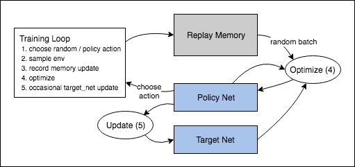
The first algorithm we tried is DQN which is an off-policy q learning algorithm. The whole workflow can be described as the following image:
PPO
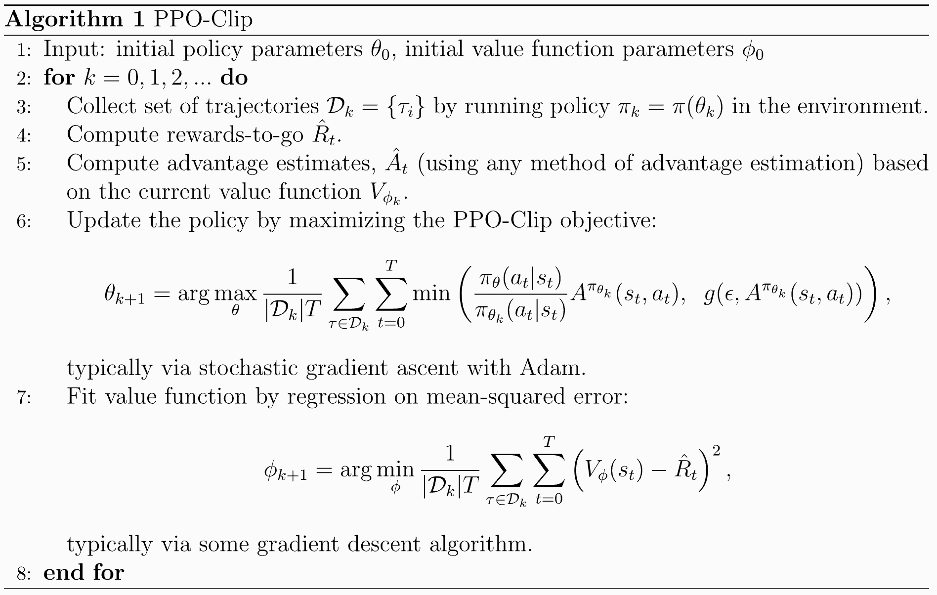
The second algorithm we tried is PPO with clipping. Below is the preudo of the algorithm. We include the detailed hyperparameters we used in the end of the post.
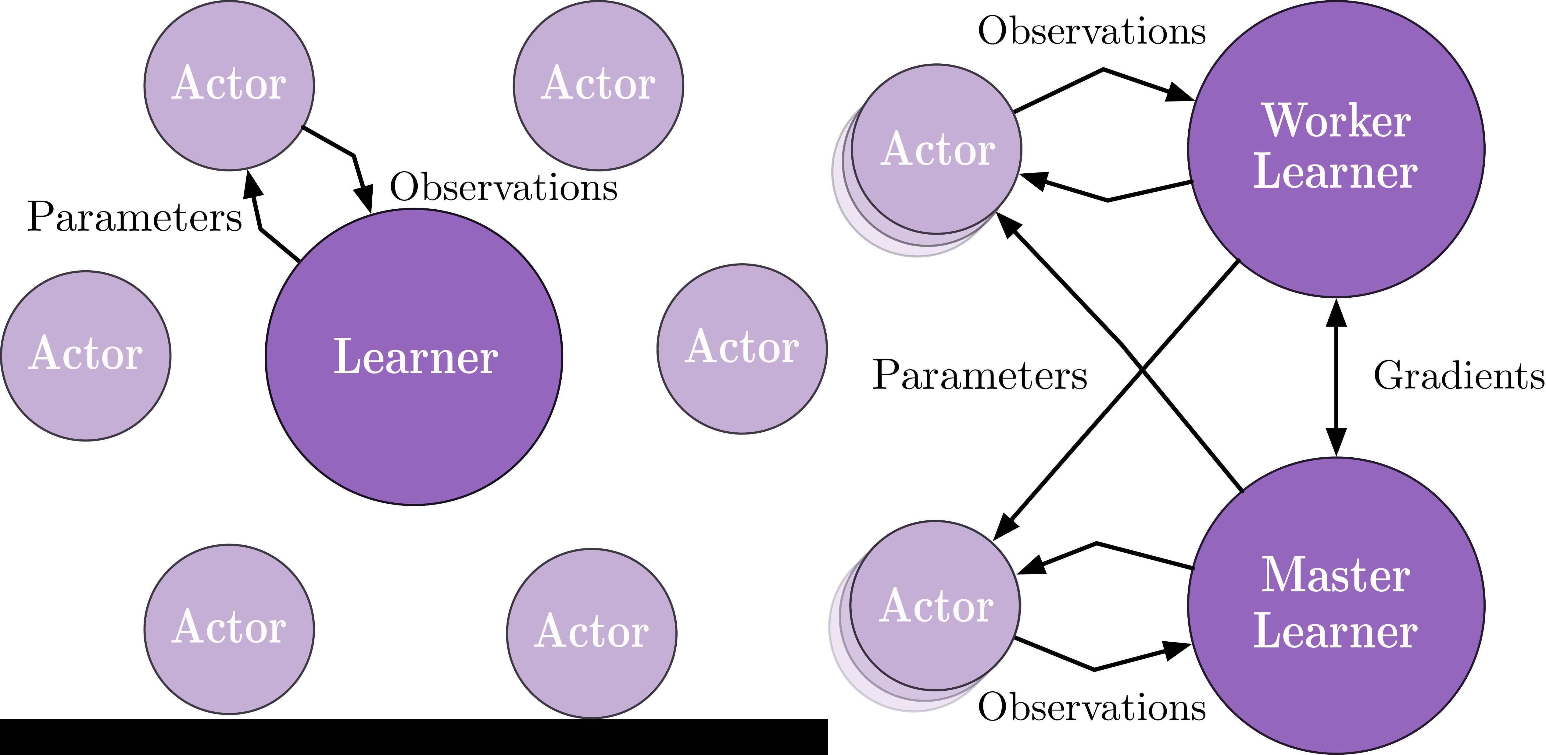
IMPALA
The last algorithm we included is IMPALA
Experiment Results
Results on 4 scenarios with different difficulty level
Here are some quick demos of applying PPO to 4 scenarios: academy_empty_goal_close, academy_run_to_score, academy_3_vs_1_with_keeper, academy_counterattack_easy.
| academy_empty_goal_close | academy_run_to_score |
|---|---|
 |
| academy_3_vs_1_with_keeper | academy_counterattack_easy |
|---|---|
 |
 |
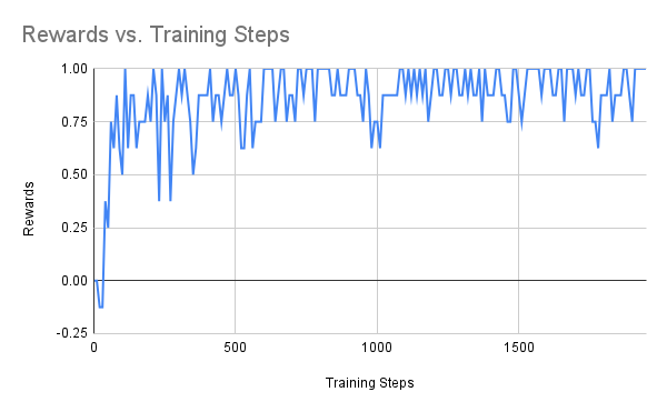
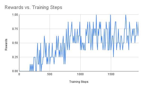
We also show their reward with respective to number of training steps
| academy_empty_goal_close | academy_run_to_score |
|---|---|
 |
| academy_3_vs_1_with_keeper | academy_counterattack_easy |
|---|---|
 |
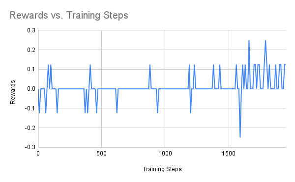 |
From the above figures, we can see that the difficulties of the scenarios increases gradually. For the players with empty goal, our agent can easily find the best action. The same happens to run to score where the scenario is also very simple. The performance fluctuation is probably due to the explorations made by the agent. For the 3 vs 1 scenario, the case is more difficult than the previous two. Our agent struggled at the very begging, but it was able to figure out the right move to achive the best rewards(scoring the goal).
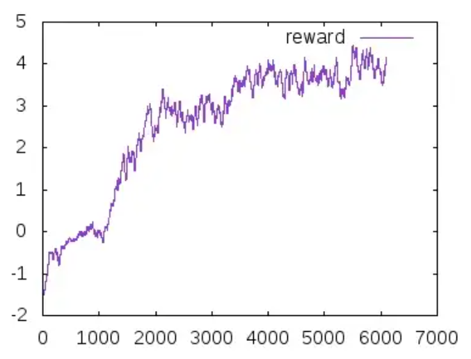
In the end, we have the most difficulty one which is to perform counter attack. In the figure above, the agents are trained for 2000 steps. As can be seen from the figure above, the agent is not able to make much progress. As we know that RL algorithms may take longer time to make progress. Therefore, I increased the number of training steps(3 times more which takes about 15 hours to finish), below is the result
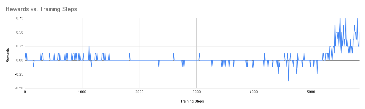 As we can see that after around 5500 training steps, the agent finally learns the right action to score goals in the counterattack scenario which justifies our assumption. Due to the time limit, we are not able to explore all of our ideas, but here are a few ideas that we want to try in the future:
- Relax the PPO clipping restriction to encourage more exploration actions
- Collect expert play history to warm up the training process such as imitation learing
Results on full match
We also try to reproduce the results for whole matches(11 vs 11). Below are the results from [1] which show the performance of different algorithms.
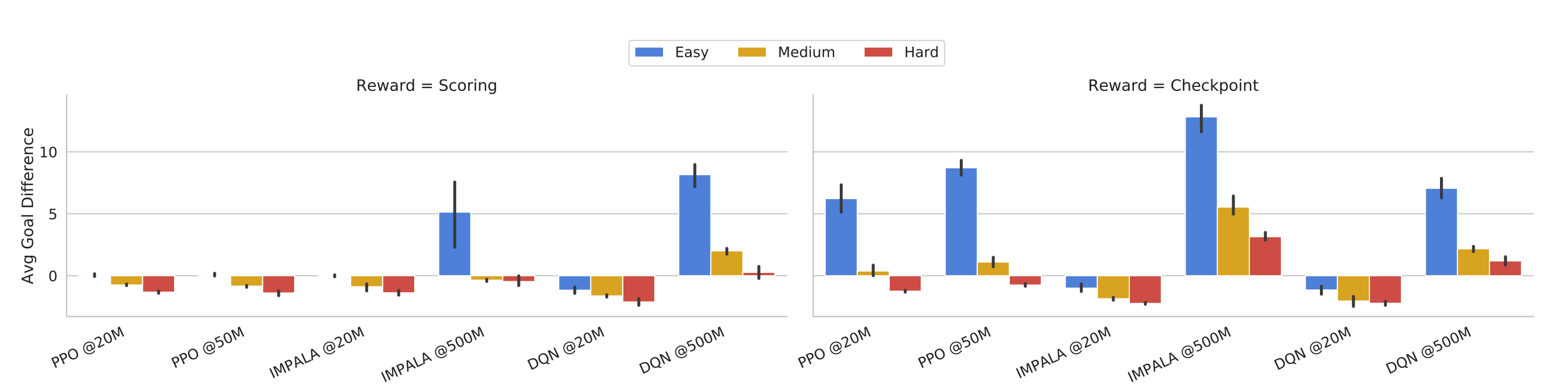 Due to the computation results, we mainly try to reprouce the results from PPO and leave the rest to future work.
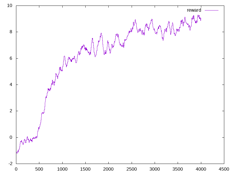
Here the x-axis is the number of steps(per 10,000 steps, e.g. 4500 means 45,000,000 steps)
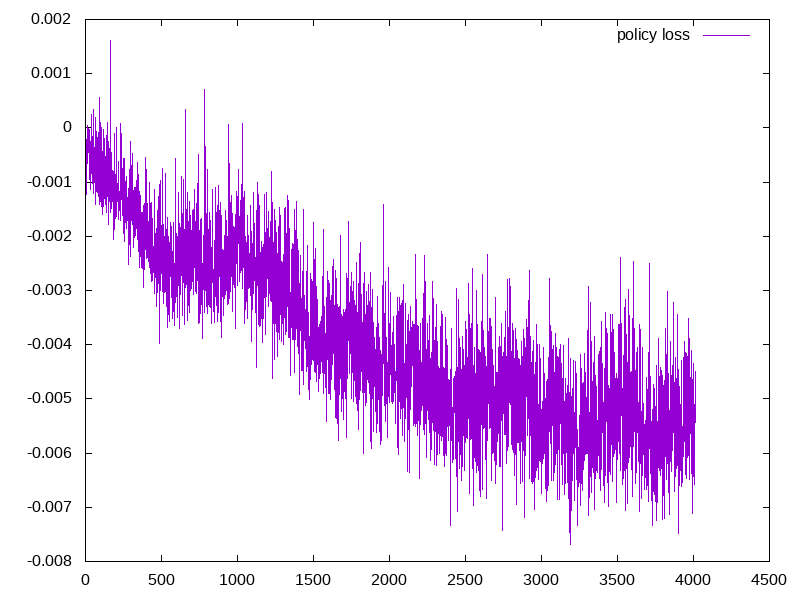
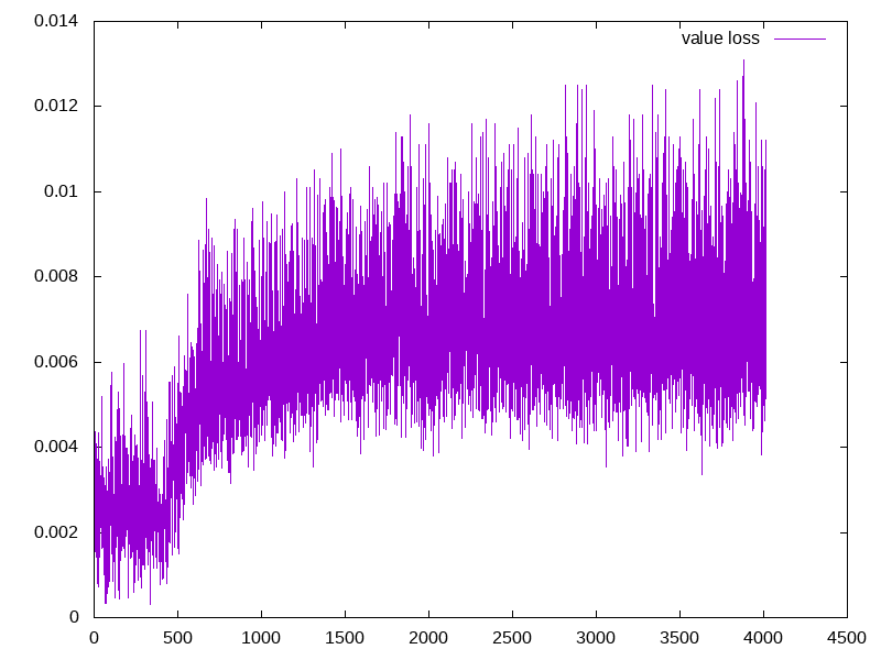
| average episode mean | policy loss | value loss |
|---|---|---|
 |
 |
 |
Below we also show the results of 2 PPO runs
| PPO run 1 | PPO run 2[2] |
|---|---|
|
 |
- It can be seen from the figures that PPO training itself is not quite stable. In our case, we are able to achive a reward of 10 within 45M steps, however in other runs, a reward of 5 can only be achieved within 50M steps.
- Another thing worth noticing is that, as the average eposide award increases, the policy loss decreases. This is expected since our agent is able to generate more useful actions. However, the value loss didn’t decrease. This is probably due to the reasons that are introduced in class that the value estimation becomes less accurate as the number of training steps increases. As a future work, we can try out the batch constrained algorithm or other techniques to see if better performance can be achieved.
- Note The runtime is very long(70 hours on a google cloud machine with around 80GB memory and A100 GPU) even if we followed the official guide. Accelerating the training process can also be one of our future directions.
One demo video of our trained agent using PPO can be seen below.
Red team is the agent which is really good after a long time of training.
🚀 Extend to real world football matches
As we know that in real world football matches, there is no way for us to directly get the complete status of the enrionment like the ones we get in the simulated environment. One way to tackle it is to combine computer vision with RL. Instead of feed the observations of GRF to the RL models(like most of other approaches), we can directly feed the game frames to the model and maximize the generability. Below are our approaches.
Input
As we are processing sequences of images(video) as input, there are multiple ways that we can design the input. One way is to feed the last N images to our model, this works very effectively for Pong, however, it’s shown to be less effective in our case. The other way is to compute the difference between current image and the past images and feed the difference to the algorithm. This turns out to be much more effective than using the past few images. In our algorithm, we will follow th latter.
Interaction with the environment
We created a wrapper class to encapsulate the interactions with the environment such as caching the reply, computing the difference, etc.
class SMMFrameProcessWrapper(gym.Wrapper):
    def build_buffered_obs(self) -> np.ndarray:
        """
        Iterate over the last dimenion, and take the difference between this obs
        and the last obs for each.
        """
        agg_buff = np.empty(self._obs_shape)
        for f in range(self._obs_shape[-1]):
            agg_buff[..., f] = self._obs_buffer[1][..., f] - self._obs_buffer[0][..., f]

        return agg_buff

    def step(self, action: int) -> Tuple[np.ndarray, float, bool, Dict[Any, Any]]:
        """Step env, add new obs to buffer, return buffer."""
        obs, reward, done, info = self.env.step(action)

        obs = self._normalise_frame(obs)
        self._obs_buffer.append(obs)

        return self.build_buffered_obs(), reward, done, info

    def reset(self) -> np.ndarray:
        """Add initial obs to end of pre-allocated buffer.

        :return: Buffered observation
        """
        self._prepare_obs_buffer()
        obs = self.env.reset()
        self._obs_buffer.append(obs)

        return self.build_buffered_obs()
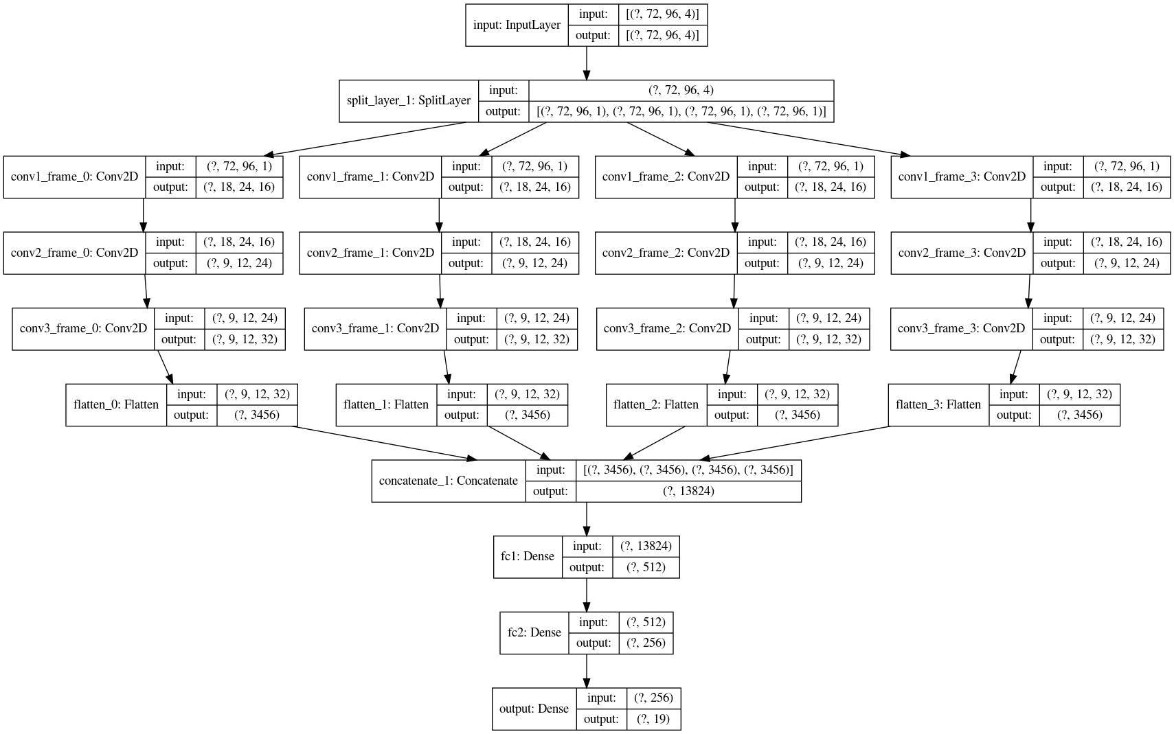
Observation processing
We use a convolutional network to process the inputs and convert them into observations. Below is an illustration of our model. As our input will be frame based, based on our experiments, it’s hard for the agent to make progress based on learning from single frames. Therefore, we extract the images from the last 4 frames and process them separately. We concatenate them together to make the final prediction.
Agent
For this approach, we start by using a DQN network as the agent. The architecture of DQN is described as below
We are currently using the implementaion from OpenAI Baseline as the baseline, below is a simple code snippet(just for demo purpose)
from baselines import deepq
import gfootball.env as football_env
from arguments import get_args

env = create_single_football_env(args)
act = deepq.learn(
    env,
    network='mlp',
    lr=1e-3,
    total_timesteps=100000,
    buffer_size=50000,
    exploration_fraction=0.1,
    exploration_final_eps=0.02,
    print_freq=10,
    callback=callback
)
Here is a simple demo of agent trained with DQN + Image frame input
 As more training data are required to train the model that directly learn from image frames, we are not able to achieve similar results as above. We leave it to future work.
Hyperparameters
For the PPO agent for 11 vs 11 we used, the final training hyperparamters are below after tuning
#!/bin/bash
python3 -u -m gfootball.examples.run_ppo2 \
  --level 11_vs_11_easy_stochastic \
  --reward_experiment scoring \
  --policy impala_cnn \
  --cliprange 0.115 \
  --gamma 0.997 \
  --ent_coef 0.00155 \
  --num_timesteps 50000000 \
  --max_grad_norm 0.76 \
  --lr 0.00011879 \
  --num_envs 16 \
  --noptepochs 2 \
  --nminibatches 4 \
  --nsteps 512 \
  "$@"
For the PPO agent for the 4 scenarios, the hyperparameters are
gamma: 0.993
num_workers: 8
batch_size: 8
learning_rate: 0.00008
epoch: 4
nsteps: 128
vloss-coef: 0.5
ent-coef: 0.01
tau: 0.95
total-frames: 2e6
eps: 1e-5
clip: 0.27
max_grad_norm: 0.5
Conclusion and Future work
It can be seen from above examples that our RL agent is able to learn how to play football by observing the stats and getting rewards. Different algorithm may fit different scenarios, e.g. PPO is very effective in both the 4 scenarios and the 11 vs 11 game plays. Also although RL agent is able to learn to play the game eventually, it can be very slow from the very beginning. Therefore, as a future work, we can explore ways to speed up the training process by imitation learning, etc. Our other future work includes testing out different backbone models and extending our RL agent to real world football matches instead of relying on the observations and states directly given by GRF(Google Research Football) directly. We believe this direction will greatly unlock the power of RL on real world football games such as the world cup.
Hardware
We used one google cloud instance with 80GB memory and one single NVIDIA A100 GPU.
Reference
[1] Kurach, K., Raichuk, A, et al. “Google Research Football: A Novel Reinforcement Learning Environment” Proceedings of the AAAI Conference on Artificial Intelligence. 2020.
[2] Lucas, Bayer, et al. “Reproducing Google Research Football RL Results”
[3] Felipe BiVORT HAIEK, “Convolutional Deep-Q learner”
[4] Scott Fujimoto, “Off-Policy Deep Reinforcement Learning without Exploration”
[5] John Schulman, “Proximal Policy Optimization Algorithms”