Multi-Agent Traffic Learning based on MARL
The project mainly focuses on the problem of traffic simulation. Concretely, this problem refers to having the agents controlled by computers learn to simulate the behavior that people will do when driving in different environments. We plan to reproduce a multiagent reinforcement learning (MARL) algorithm called Coordinated Policy Optimization (CoPo) for this problem. For the method evaluation, we plan to deploy this model to a driving simulator called MetaDrive, including five typical traffic environments, and analyze the behaviors of the individuals.
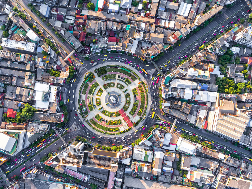 Image Credit: https://www.iskra.eu/en/Smart-traffic/Smart-roundabout/
1. Description
Traffic systems can be a kind of Self-Driven Particles systems [1]. It is hard to design manual controllers for the traffic system of vehicle flow since the interactions of agents are time-varying and the environment is non-stationary in this problem [2]. The development of multi-agent reinforcement learning (MARL) in competitive multi-player games [3, 4, 5] these years appears to provide a solution for SDP. However, there are still some challenges for it. Firstly, each constituent agent in an SDP system is self-interested and the relationship between agents is constantly changing. Second, it is difficult to generate the social behaviors of the vehicle flow through a top-down design since cooperation and competition naturally emerge as the outcomes of the self-driven instinct and the multi-agent interaction. Lastly, most of the MARL methods assume that the role of each agent is pre-determined and fixed within one episode but the agent in SDP has its individual objective [1].
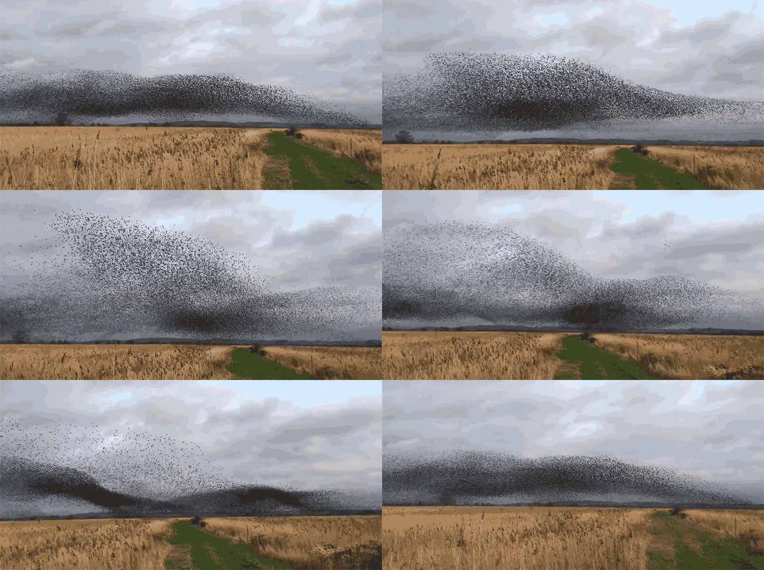 Image Credit: https://gfycat.com/
2. Method
Although MARL provides a solution to the SDP problem, there are still issues that have not been taken into account.
Firstly, each constituent agent in an SDP system is self-interested and the relationship between agents is constantly changing.
Second, it is difficult to generate the social behaviors of the vehicle flow through a top-down design since cooperation and competition naturally emerge as the outcomes of the self-driven instinct and the multi-agent interaction.
In this project, we will reproduce the research of Peng et al. [1] in the MetaDrive driving simulator [6], where they propose a novel MARL algorithm called Coordinated Policy Optimization (CoPo) for the simulation of the traffic system. This algorithm aims to control all the vehicles in the scene by operating on the low-level continuous control space.
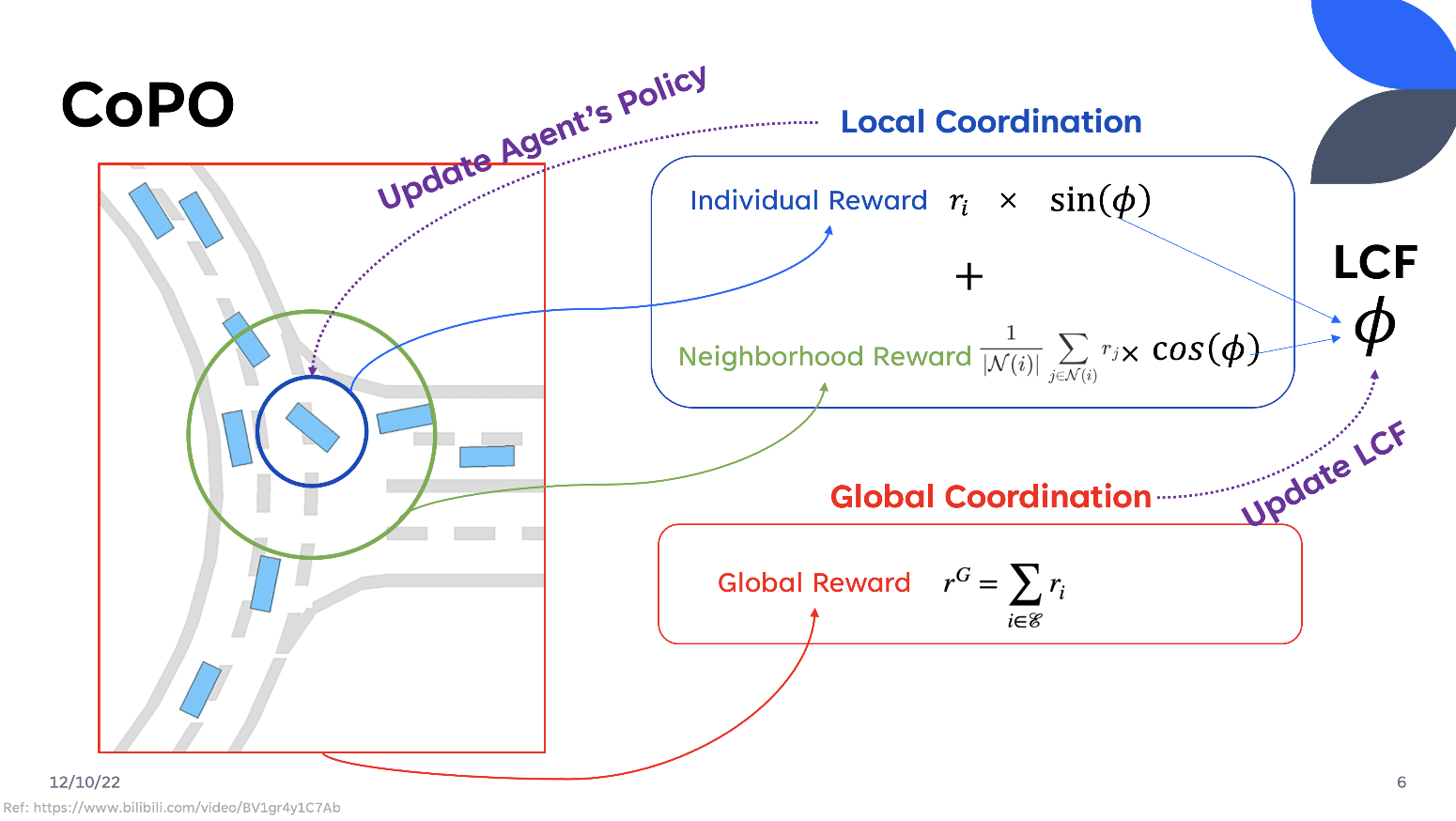
The CoPo facilitates the coordination of agents at both local and global levels. The CoPO uses PPO as the training framework and incorporates Local Coordination and Global Coordination.
Local Coordination
At the local level, CoPO takes Individual rewards \(r_{i, t}^I\) and Neighborhood reward \(r_{i, t}^N\) into account. The neighborhood is defined as follows:
\[r_{i, t}^N=\frac{\sum_{j \in \mathcal{N}_{d_n}(i, t)} r_{j, t}}{\left|\mathcal{N}_{d_n}(i, t)\right|}\]where \(r_{j,t}\) represents the individual reward of agent \(i\) at step \(t\), \(\mathcal{N}_{d_n}(i, t)\) defines the neighborhood of agent \(i\) within the radius \(d_n\).
Local Coordination utilized a Local Coordination Factor \(\phi\) (LCF), inspired by a social psychology metric named social value orientation [7], to coordinate the Individual Reward and the Reward of its Neighborhood. LCF is a degree range from -90 degrees to 90 degrees. It coordinated the Individual Reward and Global Reward as follows:
\[r_{i,t}^C = cos(\phi)r_{i,t} + sin(\phi)r_{i,t}^N\]The policy gradient is computed as [8]:
Then the PPO framework is utilized to update the policies to maximize coordinated reward. The coordinated objective is defined as follows:
\[J_i^C\left(\theta_i, \Phi\right)=\underset{(s, \mathbf{a})}{\mathbb{E}}\left[\min \left(\rho A_{\Phi, i}^C, \operatorname{clip}(\rho, 1-\epsilon, 1+\epsilon) A_{\Phi, i}^C\right)\right]\]where \(A_{\Phi, i}^C = cos(\phi)A^I_{i,t} + sin(\phi)A^N_{i,t}\) is the coordinated advantage function, LCF \(\phi\) is a random variable which follows the distribution \(\mathcal{N}(\phi_\mu, \phi^2_\sigma)\), and \(\Phi=[\phi_\mu, \phi_\sigma]^\top\) are learnable parameters for LCF distribution.
Global Coordination
The LCF here will affect the agent’s preference of being selfish (\(\phi = 0°\)) or selfless (\(\phi = 90°\)). However, there is still a serious problem how can we determine the LCF? It is always difficult to find the best value manually which requires a lot of parameter tuning in the training process each time.
The CoPO designs a Global Coordination to adjust LCF as a learnable parameter. At Global Coordination, they design a global reward, which is the sum of the reward of all agents at all steps, and the global objective is defined as follows:
\[J^G\left(\theta_1, \theta_2, \ldots\right)=\underset{\tau}{\mathbb{E}}\left[\sum_{i \in \mathcal{E}_\tau} \sum_{t=t_i^s}^{t_i^e} r_{i, t}\right]=\underset{\tau}{\mathbb{E}}\left[\sum_{t=0}^T \sum_{i \in \mathcal{E}_{\tau, t}} r_{i, t}\right]\]where \(\mathcal{E}_{\tau, t}\) denotes the active agents in the environment at step \(t\).
Then, the global coordination computes the gradient of the global objective with respect to LCF, to update and optimize LCF by introducing the individual global objective :
\[J^{LCF}(\Phi)=\underset{i,(s, \mathbf{a}) \sim \theta^{\text {old}_i}}{\mathbb{E}}\left[\nabla_{\theta_i^{\text {new }}} \min \left(\rho A^G, \operatorname{clip}(\rho, 1-\epsilon, 1+\epsilon) A^G\right)\right]\left[\nabla_{\theta_i^{\text {old }}} \log \pi_{\theta_i^{\text {old }}}\left(a_i \mid s\right)\right] A_{\Phi, i}^C\]Therefore, we can conduct gradient ascent on \(J^{LCF}\) with respect to \(\Phi\).
3. Experiments
Installation
We have installed the MetaDrive according to the MetaDrive Github README on Ubuntu 18.04. The Single Agent Environment and Multi-Agent Environment from different scenarios in MetaDrive are tested.
We installed CoPO and setup a GPU-supported enviroment in Linux according to https://github.com/decisionforce/CoPO.
Training & Evaluation
Due to the limitations of memory and computational resources on our PC, we modified the training mode to local, using single-thread and removing grid search, following the instructions given in the FAQ on CoPO’s GitHub page. We trained CoPO in the Intersection and Roundabout environment, following the example modified code for IPPO local training with GPU acceleration. We also modified the number of agents to 20 for accelerating the model performance on our PC.
The training curves of Intersection and Roundabout environment are shown as follows:

The trained models are evaluated on 20 episodes and their success rates are 85.67% in the Intersection environment and 88.07% in the Roundabout environment.
Visualization
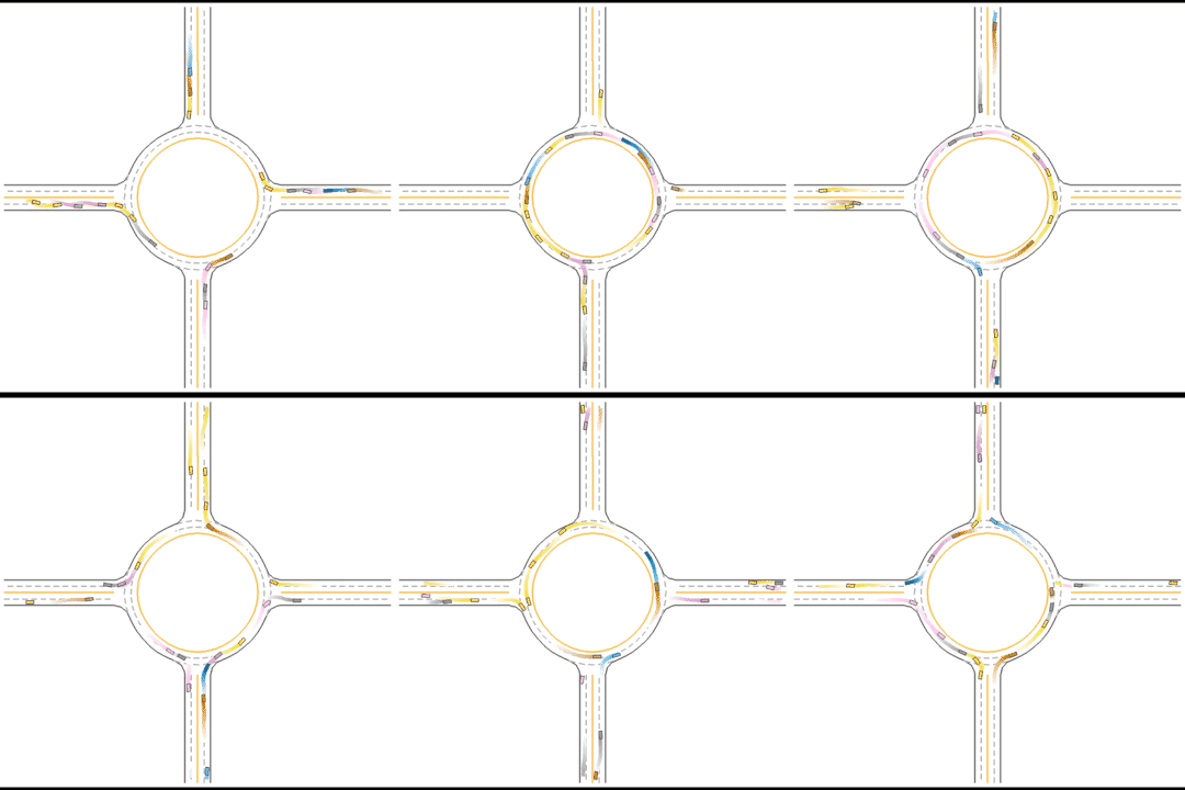
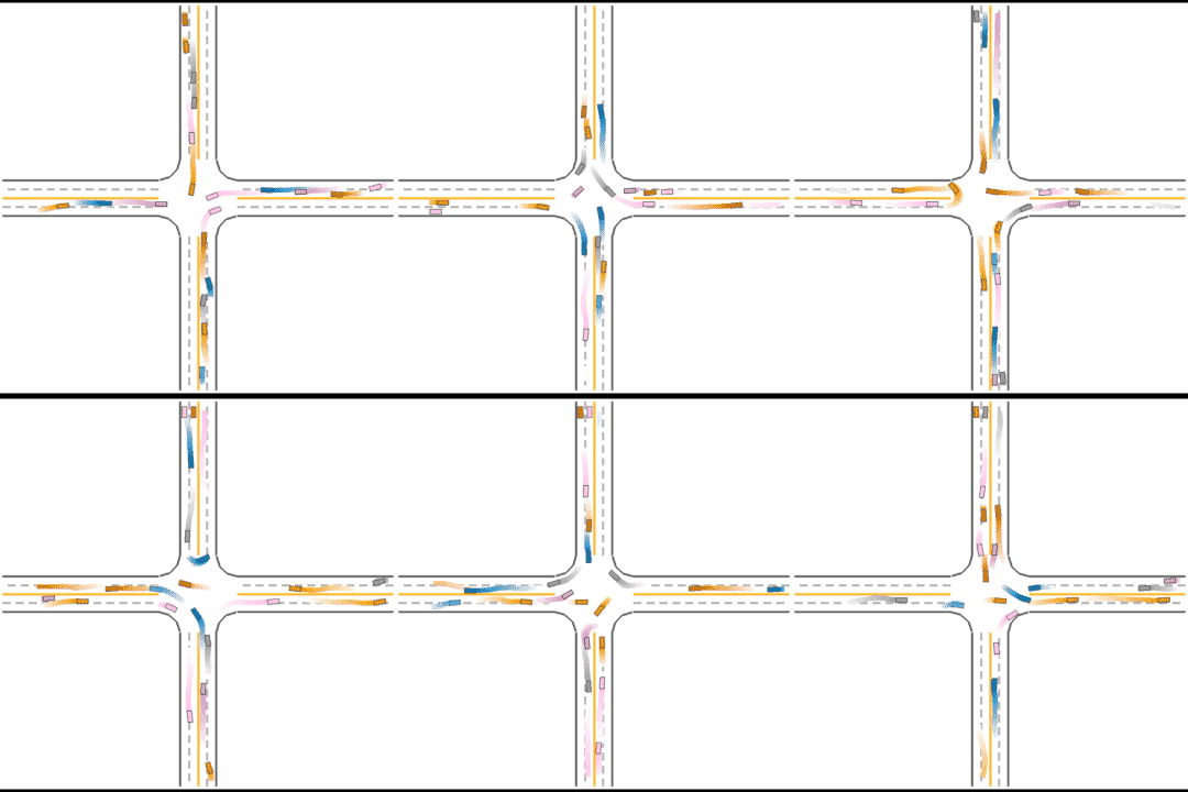
We also visualized the behaviors of the populations during the training process to observe their learning processes.
At first, these agents appear to basically have no idea how to drive.
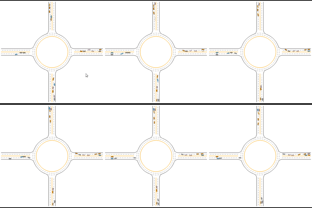
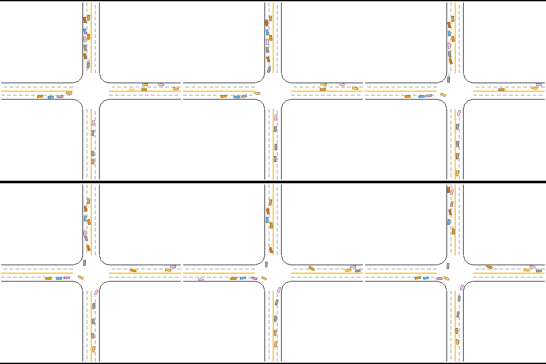
Gradually, they learned how to drive in simple scenarios but were still overwhelmed by the complex ones.
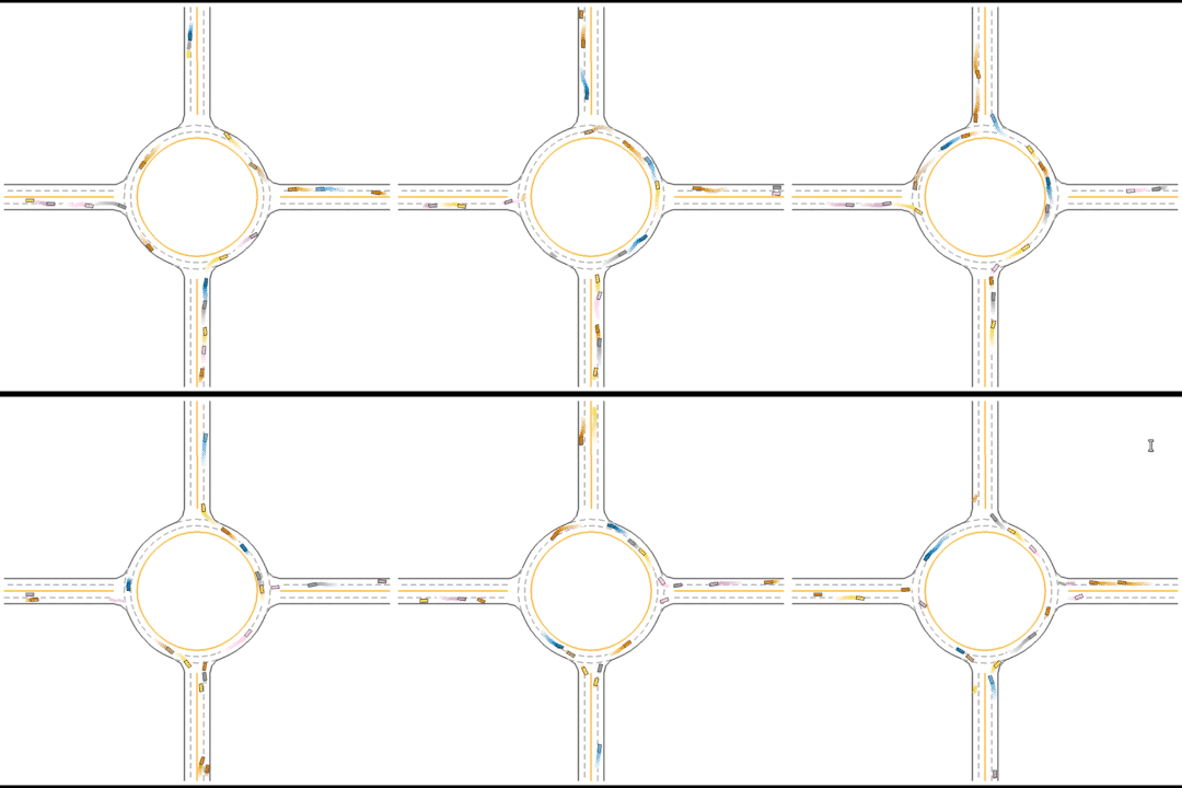
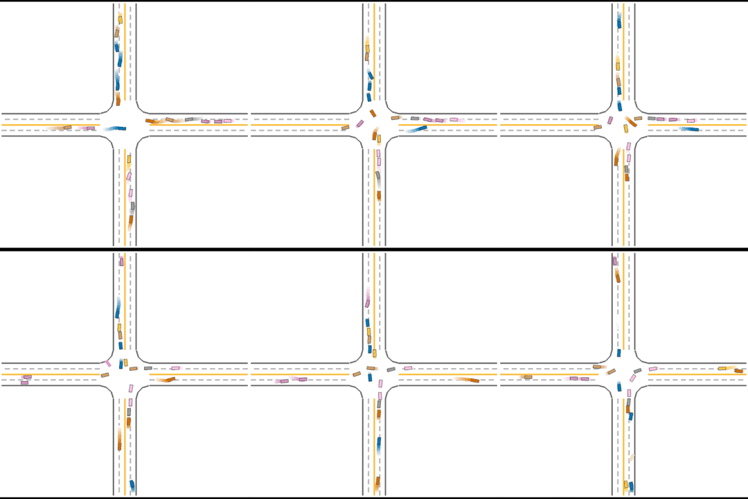
They continue to improve their driving ability, but they don’t seem to know how to handle some situations safely.
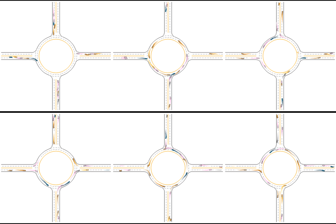
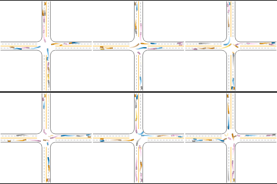
Finally, they seem to have mastered some human driving behaviors, including queueing, yielding, and cutting in.
Impacts of Parameters
We further evaluate the impacts of some parameters and plot some figures in this section.
Number of Agents
Firstly, we evaluate the impact of the number of agents. The training curves on the Intersection Environment and Roundabout Environment are shown as follows.
In general, as the number of agents increases, the rises of success rate taking more time steps. Except that when the number of agents is 5, the success rate seems to stagnate for a while, but then it rises at the max rate.