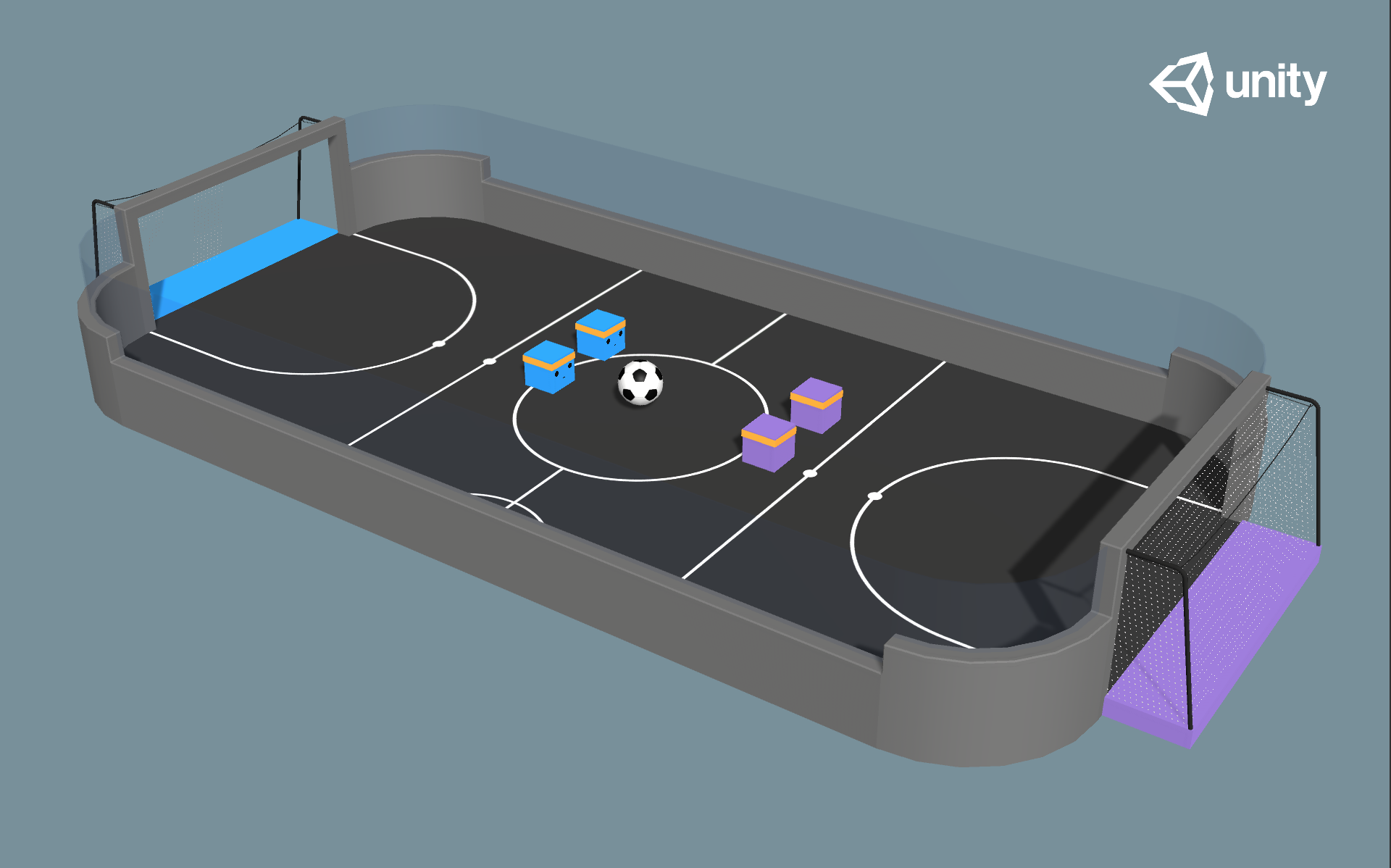
2 vs 2 soccer game
In this project we are going to investigate Multi-Agent Reinforcement Learning (MARL). Unlike vanilla RL tasks, MARL involves training multiple agents to learn and make decisions based on their interactions with both the environment and other agents. To illustrate the potential of MARL, we build a 2 vs 2 soccer game in Unity and apply different MARL algorithms to it. We then use the ELO score to evaluate the performance of the multi-agent algorithms and compare them to single-agent algorithms running on MA systems. In the end, we design a fighting experiment where two agents trained by different algorithms play against each other and clearly demonstrate how their behavior varies.
- We want to play Soccer two by AI !
- What is MARL?
- Environment Specified Challenges and Solution
- Related Work
- Methodology and Algorithms
- Soccer Two Spec
- Experiments & Results
- Fight time
- Conclusion
- Future Work
- Source code
- Implementation
- Results
- References
We want to play Soccer two by AI !
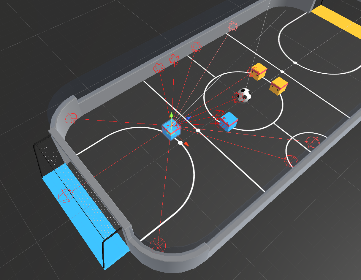
We are working on a 2 vs 2 soccer game in Unity (as shown in Fig. 0). In this game, there are two teams with two agents in each. The goal is to get the ball into the opponent’s goal while preventing the ball from entering own goal.
Traditional RL algorithms such as DQN or PPO face several challenges when adapted to multi-agent settings, those challenges include:
- Nonstationarity: One of the biggest challenges facing MA systems is the nonstationary nature of the environment seen by each agent. As the policies of other agents evolve, the dynamics of the environment change over time, making it difficult for agents to learn and make decisions effectively.
- Exponential growth The action space grows exponentially with the number of agents.
- Cooperative vs. Competitive When there are both cooperative and competitive agents, the overall problem becomes a minimax optimization problem, which has complex cycling behavior instead of simple min or max optimization.
Therefore, we need to develop MARL technologies to solve problems arising from multi-agent interactions.
What is MARL?
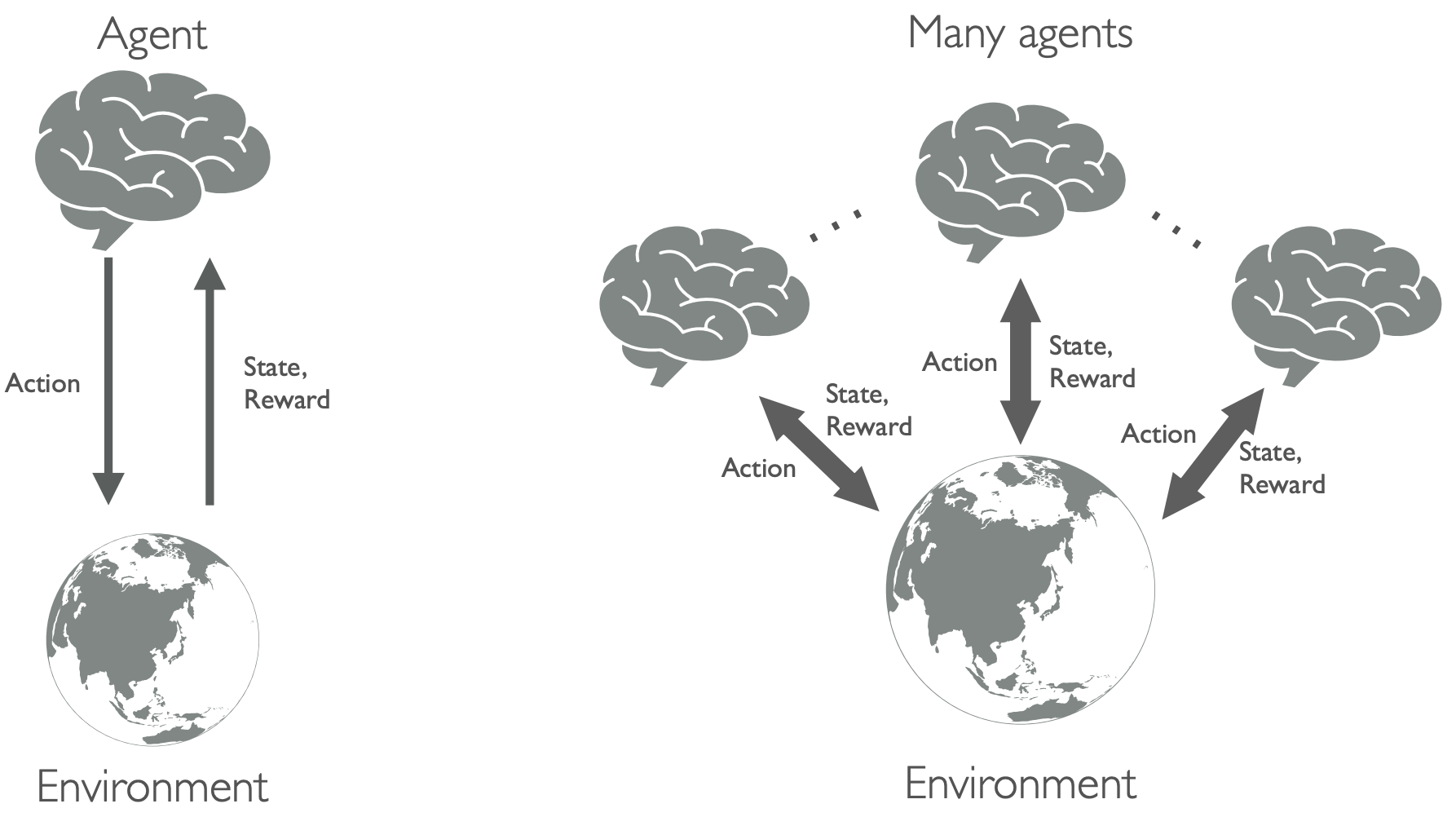
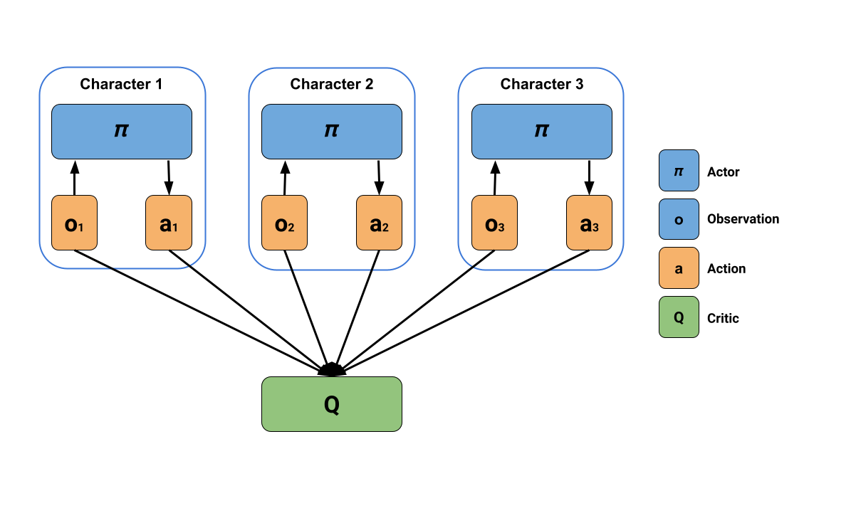
Different from single-agent systems, in multi-agent systems, the environment and the rewards received by each agent are not only determined by the environment itself, but also by the joint actions of other agents. As a result, agents must take into account and interact with not only the environment, but also with other intelligent agents (see Fig. 1). In a multi-agent scenario, there can be cooperation (e.g., May and Cody in video game It Takes Two) and competition (e.g., most of board games) between agents. Next, we introduce the main techniques that we are considering in this blog.
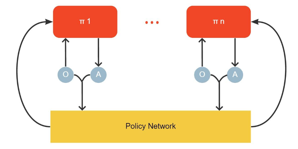
Cooperative training Basic ML training techniques includes independent learners, where we train each agent independently with each other; sharing parameters, where all agents in one team uses their own observations and locations to train a single policy network; centralized critic, where agents are trained independently via actor-critic techniques while the critic are trained using global information; value function factorization, that solves the problem of lazy agents by distributing the global reward among the agents; consensus, that reduces communication costs hrough sparse network communication and achieves consensus.
Self-play for competitive training Training agents to perform complex competitive tasks requires high complexity of the environment, which is in general hard to achieve in regular training environments. Self-play is a concept in which an opponent agent provides diversified responses to a trained agent, allowing it to learn complex tasks in a complex environment. This concept has been used in games such as AlphaGo and Dota2, and can be traced back to TD-gammon. In a self-play game, the opponent agent also provides the trained agent with the right curriculum to learn.
Environment Specified Challenges and Solution
In a soccer game, agents must adapt to changing positions and actions of both teammates and opponents to maximize rewards. This makes Soccer Two a challenging environment for MARL algorithms, and a useful testbed for studying the capabilities and limitations of different MARL approaches.
In this environment, we mainly have the following question:
- How to control the role separately?
A challenge that we are facing in training for the two-soccer game is that we need to train more than one brain at a time, e.g. there is a goalie that needs a defensive brain and a striker that needs an offensive brain. So we need different reward functions to train different controllers. By enabling the multi-brain training feature in the ML-Agents toolkit of Unity, we are building our algorithms based on not only a two-player setting, but also each player has two brains present. After training, we get one neural network model for each brain, that further enables mixing and matching different hyperparameters.
- How to train the antagonism between both sides?
Since there could exist a situation that two-side players do not move all the time that making the game meaningless, it is important to consider how to train the adversarial between two players, we propose to experiment with using the self-play technique to enhance the performance. We will analyze how the two-brain setting affects the training, as well as how the self-play affects the training, etc.
Related Work
We list some related MARL papers here, and interested readers can refer to these articles for a more complete understanding of the literature.
- Independent Learning
- Value Decomposition
- Policy Gradient
- Communication
- BiCNet:Multiagent Bidirectionally-Coordinated Nets: Emergence of Human-level Coordination in Learning to Play StarCraft Combat Games [10]
- CommNet:Learning Multiagent Communication with Backpropagation [11]
- IC3Net:Learning when to Communicate at Scale in Multiagent Cooperative and Competitive Tasks [12]
- RIAL/RIDL:Learning to Communicate with Deep Multi-Agent Reinforcement Learning [13]
- Exploration
- Self-play
Methodology and Algorithms
In this section, we introduce the methodology of several algorithms that we add to our analysis. We start from the single-agent algorithm PPO, and then move on to introduce other extensions of policy gradient and actor-critic based approaches, as well as their design for multi-agent environments.
PPO
For policy gradient algorithms, the update on the policy parameters equals to taking approximate gradient on an objective function, which is done by calculating a weighted gradient ascent:
\[\nabla_\theta J(\theta)=E_{s \sim \rho^\pi, a \sim \pi_\theta}\left[\nabla_\theta \log \pi_\theta(a \mid s) Q^\pi(s, a)\right]. \tag{1}\]Proximal Policy Gradient (PPO) is designed to take cautious steps to maximize the improvement. While a previous work TRPO uses complex second-order methods to solve this problem, PPO is first-order method that enables the use of gradient descent. This allows for more efficient optimization and helps to avoid performance collapse. A truncated version of the PPO objective are illlustrated as follows:
\[\min \left(\frac{\pi_\theta(a \mid s)}{\pi_{\theta_k}(a \mid s)} A^{\pi_{\theta_k}}(s, a), \operatorname{clip}\left(\frac{\pi_\theta(a \mid s)}{\pi_{\theta_k}(a \mid s)}, 1-\epsilon, 1+\epsilon\right) A^{\pi_{\theta_k}}(s, a)\right).\]MAPPO (Multi-Agent Proximal Policy Optimization) is an actor-critic algorithm in which the critic learns a joint state value function. MAPPO can utilise the same training batch of trajectories to perform several update epochs.
DDPG
The deterministic policy gradient (DPG) is based on continuous and deterministic policy hypothesises \(\mu_{\theta}(s): {S} \rightarrow {A}\) (in comparison with \(\pi_{\theta}(s \mid a)\) which is a probability distribution). Instead of using (1), the objective gradient of DPG yields:
\[\nabla_\theta J(\theta)=E_{s \sim \beta}\left[\left.\nabla_\theta \mu_\theta(s) \nabla_a Q^\mu(s, a)\right|_{a=\mu_\theta(s)}\right]. \tag{2}\]Based on DPG formular (2), DDPG is an actor-critic based algorithm that trains a value network and a policy network, and leverages DQN training techniques such as the experience replay, and the target network. Next we introduce adding a multi-agent structure on top of DDPG.
MADDPG
Motivation One major challenge of using traditional reinforcement learning (RL) techniques in multi-agent settings is that the constant learning and improvement of each agent’s strategy interferes with the environment and makes it highly unstable from the perspective of each individual agent. This instability violates the convergence conditions of traditional RL algorithms, making RL algorithms difficult to use in multi-agent scenarios. Furthermore, policy gradient-based algorithms also suffer from high variance in multi-agent environments, which is exacerbated by the increasing number of agents. To address these challenges, the Multi-Agent Deep Deterministic Policy Gradient (MADDPG) algorithm has been designed with specific characteristics to improve its performance in multi-agent settings.
Approach In 2017, OpenAI introduced the Multi-Agent Deep Deterministic Policy Gradient (MADDPG) algorithm in their paper “Multi-Agent Actor-Critic for Mixed Cooperative-Competitive Environments”. MADDPG (Multi-Agent Deep Deterministic Policy Gradient) is a variation of the DDPG algorithm for MARL, extending DDPG into a multi-agent policy gradient algorithm where decentralized agents learn a centralized critic based on the observations and actions of all agents. The action space of MADDPG must be continuous due to the differentiability of actions with respect to the parameters of the actor. After, Lowe et al. apply the Gumbel-Softmax trick to learn in discrete action spaces.
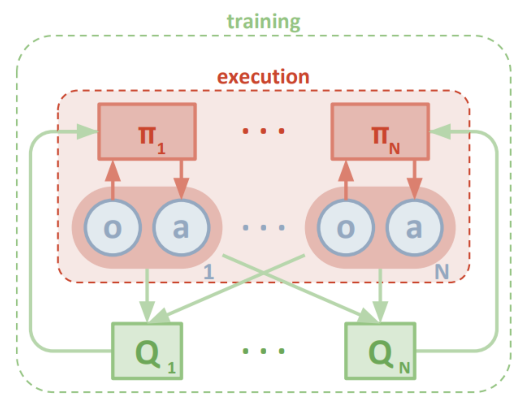
As illustrated in Fig 4. The actor is conditioned on the history of local observations, while the critic is trained on the joint observation and action to approximate the joint state-action value function. Each agent individually minimizes the deterministic policy gradient loss. After training is completed, only the local actors are used in the execution phase, acting in a decentralized manner.
Specifically, the “decentralized actor” updates are similar as that used in DDPG (2), we formulate it as follows:
\[\nabla_{\theta_i} J\left(\mu_i\right)=E_{x, a \sim D}\left[\left.\nabla_{\theta_i} \mu_i\left(a_i \mid o_i\right) \nabla_{a_i} Q_i^\mu\left(x, a_1, \cdots, a_n\right)\right|_{a_i=\mu_i\left(o_i\right)}\right]\]for the continuous policy case, or
\[\nabla_{\theta_i} J\left(\theta_i\right)=E_{s \sim \rho^\pi, a_i \sim \pi_i}\left[\nabla_{\theta_i} \log \pi_i\left(a_i \mid o_i\right) Q_i^\pi\left(x, a_1, \cdots, a_n\right)\right]\]for the discrete case.
In contrast to the \(Q^\pi\) in (1) and \(Q^\mu\) in (2), policy gradient objective in MADDPG are trained with the guidence of the centralized critic \(Q_i^\pi\) or \(Q_i^\mu\), which provides information of the whole system.
On the other hand, the “centralized critic” is trained via
\[L \left(\theta_i\right)=\mathbb{E}_{\mathbf{x}, a, r, \mathbf{x}^{\prime}}\left[\left(Q_i^{\boldsymbol{\mu}}\left(\mathbf{x}, a_1, \ldots, a_N\right)-y\right)^2\right]\] \[y=r_i+\left.\gamma Q_i^{\boldsymbol{\mu}^{\prime}}\left(\mathbf{x}^{\prime}, a_1^{\prime}, \ldots, a_N^{\prime}\right)\right|_{a_j^{\prime}=\boldsymbol{\mu}_j^{\prime}\left(o_j\right)}\]With the centralized critic that utilizes global information, the training becomes more stable even if each agents are acting in a non-stationary manner.
MA-SAC
MA-SAC (Multi-agent Soft Actor-Critic) supports efficient off-policy learning and addresses credit assignment problem partially in both discrete and continuous action spaces. MASAC uses the optimization goal of maximum entropy to make the algorithm more stable. Each agent in MASAC uses an independent critic network to calculate the Q value of all states and actions, making the algorithm can be applied in a mixed collaborative and competitive environment
As shown in Figure 5, the agent \(i\) in MASAC has 4 deep neural networks, which are actor network, critic network, target actor network, and target critic network. In the training process, only the actor network and critic network are trained. The target actor network and target critic network are used to stabilizing the learning effect of the actor network and critic network. The actor network and target actor network respectively utilize the current observation \(o_i\) of the agent and the observation of the next state \({o_i}^{'}\) to generate the current action and target action.
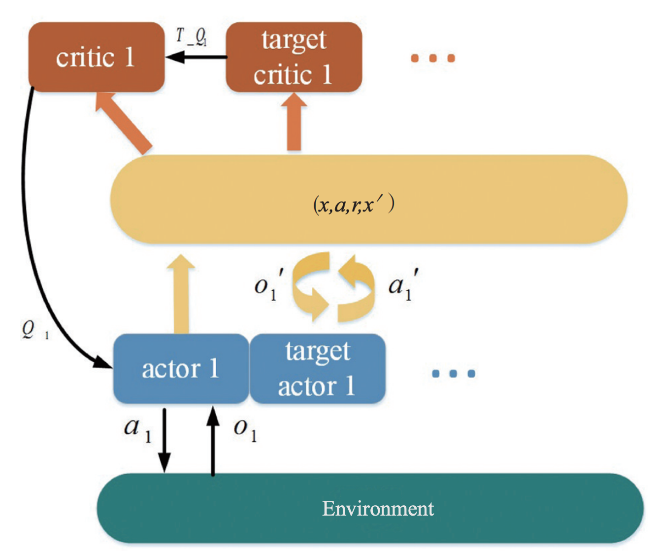
The input of critic network is the observation \(x\) and the action \(a\) of all the current agents, and the output is the Q value of agent \(i\) action, \(Q_i\). The input of target critic network is the observation \(x'\) and action \(a'\) of the agent in the next state, and the output is the Q value of agent \(i\) ‘s target action, \(T_{Q_i}\). Meanwhile, every time the parameters of actor network and critic network are updated, it will soft update target actor network and target critic network ensuring the stable operation of the algorithm.
MA-POCA
MA-POCA (Multi-Agent POsthumous Credit Assignment) is a neural network that acts as a “coach” for a whole group of agents. Since Muti-Agent game needs to be considered with functionality for training cooperative behaviors - i.e., groups of agents working towards a common goal, where the success of the individual is linked to the success of the whole group. In such a scenario, agents typically receive rewards as a group. You can give rewards to the team as a whole, and the agents will learn how best to contribute to achieving that reward. Agents can also be given rewards individually, and the team will work together to help the individual achieve those goals.
During an episode, agents can be added or removed from the group, such as when agents spawn or die in a game. If agents are removed mid-episode (e.g., if teammates die or are removed from the game), they will still learn whether their actions contributed to the team winning later, enabling agents to take group-beneficial actions even if they result in the individual being removed from the game (i.e., self-sacrifice). MA-POCA can also be combined with self-play to train teams of agents to play against each other.
Soccer Two Spec
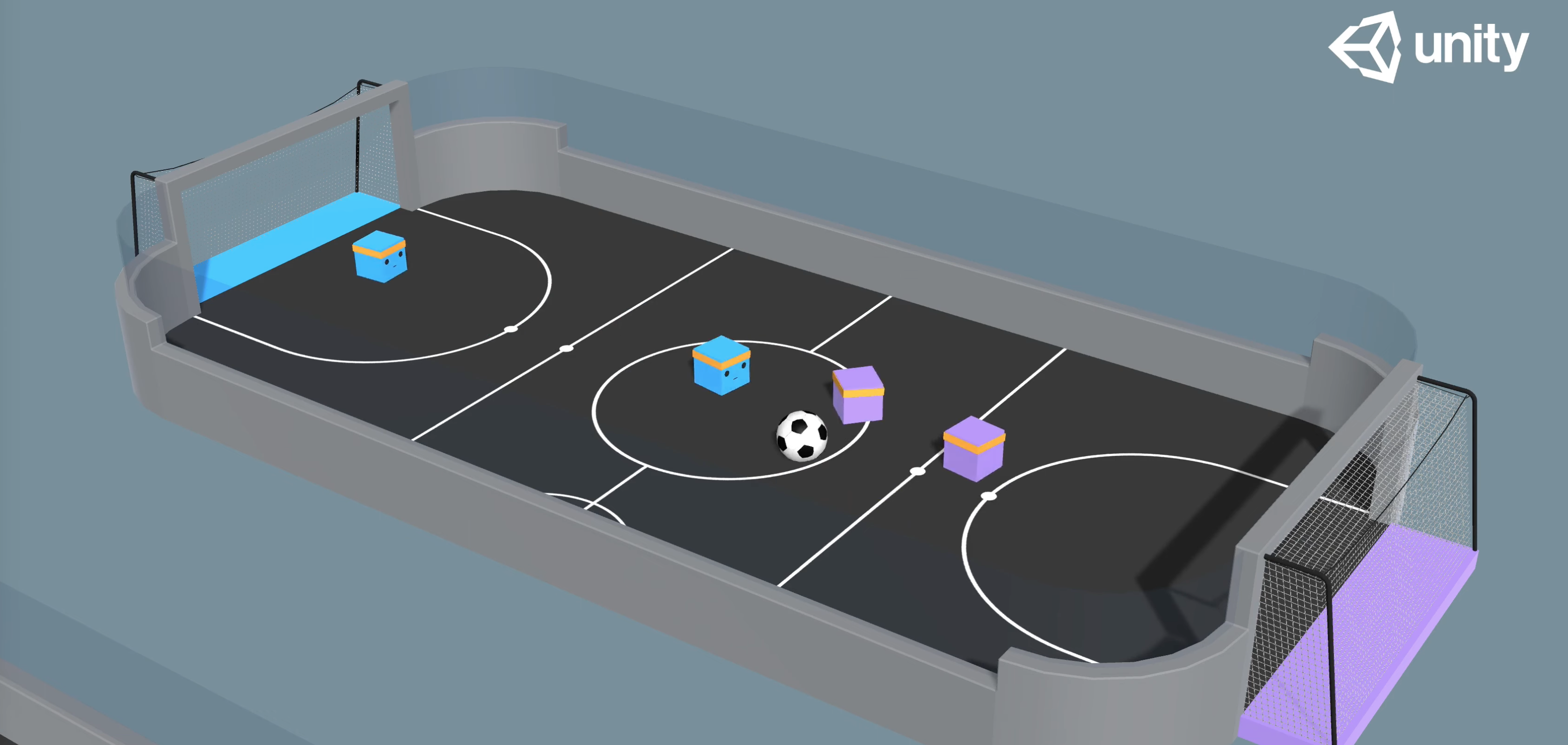
The environment is based on Unity ML Agents’ Soccer Twos, so most of the specs are the same. Here, four agents compete in a 2 vs 2 toy soccer game, aiming to get the ball into the opponent’s goal while preventing the ball from entering own goal.
-
Goal: Get the ball into the opponent’s goal while preventing the ball from entering own goal.
- Agent Reward Function:
1 - accumulated time penalty: when ball enters opponent’s goal. Accumulated time penalty is incremented by(1 / MaxSteps)every fixed update and is reset to 0 at the beginning of an episode. In this build,MaxSteps = 5000.-1: when ball enters team’s goal.
-
Observation space: 336 corresponding to 11 ray-casts forward distributed over 120 degrees (264) and 3 ray-casts backward distributed over 90 degrees each detecting 6 possible object types, along with the object’s distance. The forward ray-casts contribute 264 state dimensions and backward 72 state dimensions.
- Action space: 3 discrete branched actions (MultiDiscrete) corresponding to forward, backward, sideways movement, as well as rotation (27 discrete actions).
Experiments & Results
In this section, we demonstrate our training results on the Soccer Two environment we introduced in previous sections. We first show how our models perform under various metrics and provide detailed analysis of the results. For algorithms without self-play, we treat the system as a 2-player game and train each agent’s decisions as independent with each other. For algorithms with self-play, we take a different approach. We train one side of the game, and periodically syncronize the other side with a previous copy of the trained team. This allows the agents to compete with its own policies. By using self-play, we aim to improve the performance of our models and better capture the complex dynamics of the Soccer Two environment.
However, we note that the metrics in our setting is different from traditional supervised learning metrics in two aspects:
- The training loss decay does not directly indicate the improvement in performance in an RL environment, where the data distribution is constantly changing. In such a dynamic environment, neither the policy loss nor the critic loss is directly correlated with the performance of the policy. In other words, a decrease in the training loss does not necessarily mean that the policy is performing better. To accurately evaluate the performance of the policy, other metrics must be used.
- The episode reward does not have a meaningful interpretation in our setting, as both sides of the game are constantly improving their policies. This means that the total episode reward should be around 0 at all times, as the performance of one side is balanced out by the performance of the other side.
Therefore, to accurately evaluate the performance of our models, we need to use other metrics that are more relevant to the Soccer Two environment.
Preliminary training results
We start with some preliminary training experiments. By conducting these initial experiments, we can gain a better understanding of the challenges and opportunities presented by this complex and dynamic environment.
PPO
We first trained a simple PPO agent and observed that the episode reward has no meaning. Therefore, we changed the evaluating metrics to the entropy of the policy and the ELO in this experiment, and will present the results in later sections.
MADDPG and MA-SAC
We observe that these two models are hard to train in practice (very slow). For example, Fig 7 (top) shows the training curve of MADDPG when trained on only one agent with the opponent set as random, and Fig 7 (right) shows the training curve for self-played MADDPG. Neither obtains satisfactory results in reasonable time.
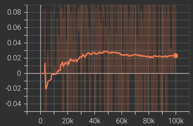
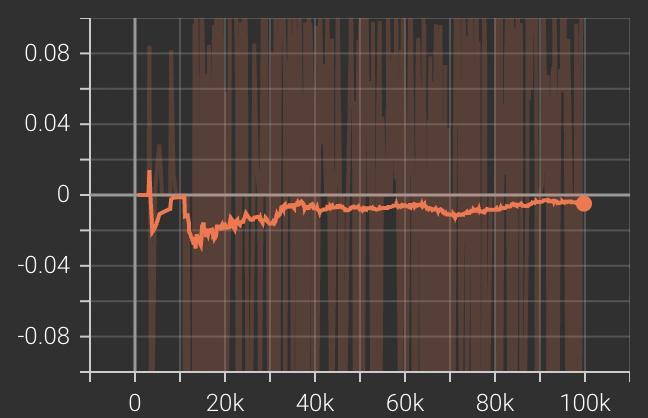
In addition, according to some recent studies, PPO with parameter sharing has been shown to outperform MADDPG in many environments [7]. So we decide to use PPO to compare with other trained agents.
MAPOCA
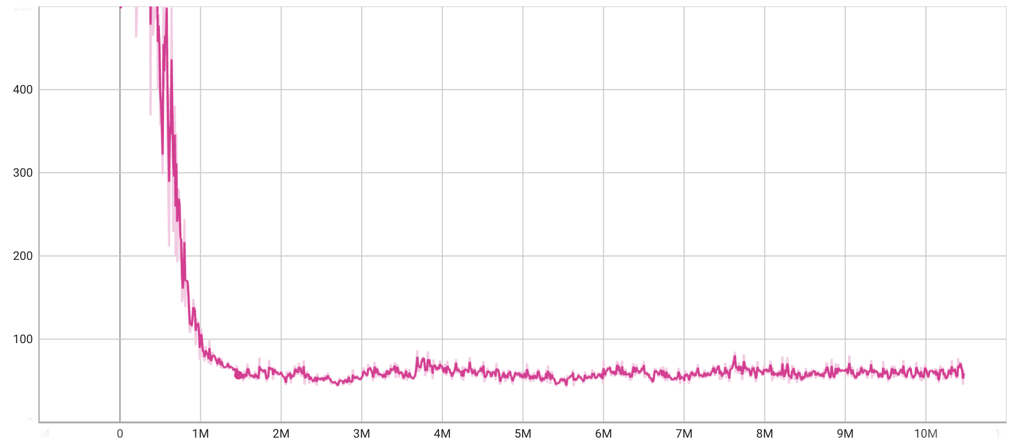
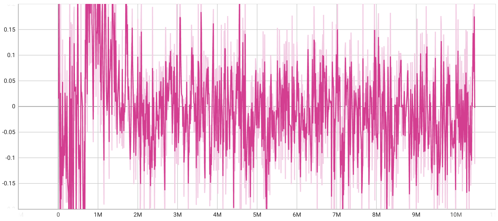
The training curve of the POCA algorithm on the two-player soccer game environment is shown in the next figure. Fig 8 (top) shows the episode length and Fig 8 (down) shows the group cumulative rewards. The reward fluctuates around 0 but the episode length is decreasing, indicating a faster goal speed.
Evaluate the Performance
In this subsection, we demonstrate the performance of our final trained agents in terms of policy entropy and ELO (Elo rating system).
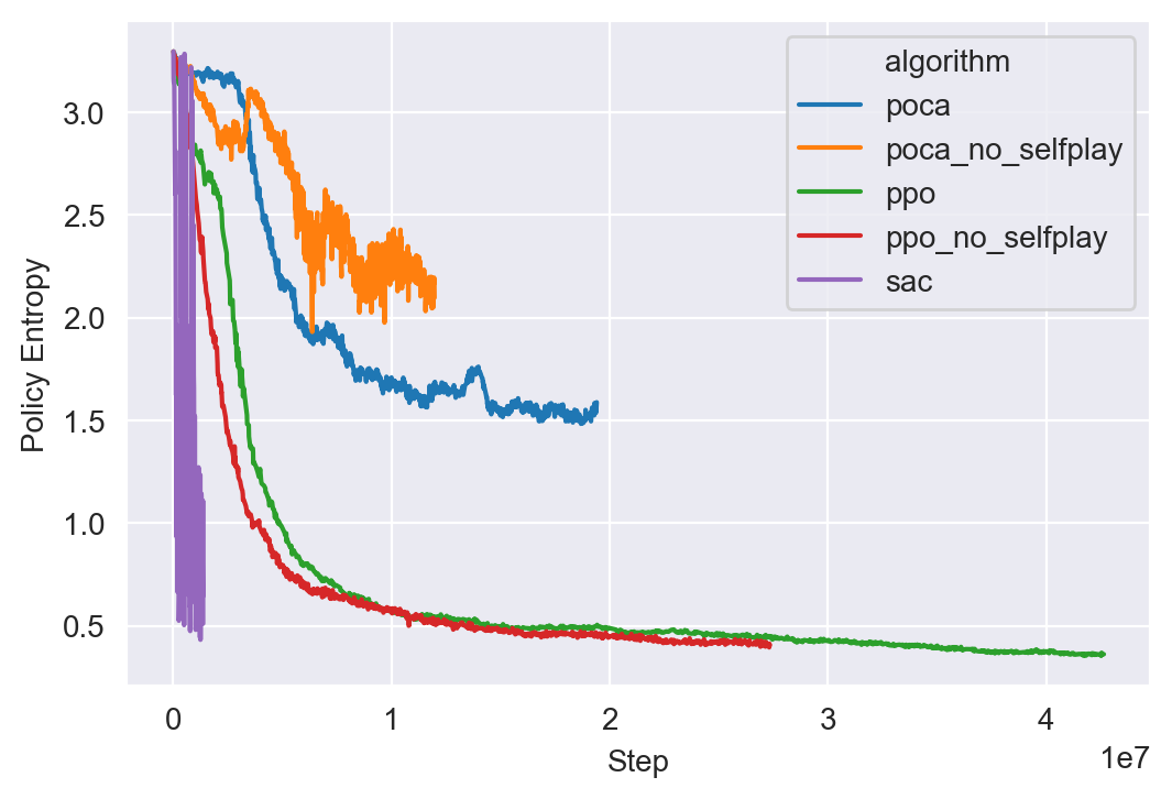
- Policy entropy is a measure of the randomness or unpredictability of an agent’s actions. A low entropy policy indicates that the agent is taking deterministic actions, while a high entropy policy indicates that the agent is taking more random or varied actions.
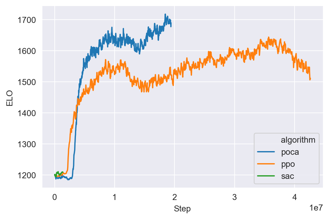
- ELO, or Elo rating system, is a method for calculating the relative skill levels of players in two-player games such as chess. It is based on the assumption that the outcome of a game is a function of the relative skill levels of the players. In our setting, it is a more effective indicator of the agents’s performance.
We list the corresponding color of the algorithms as follows: (1) Gray: MA-POCA (2) Blue: MA-PPO (3) Pink: SAC (4) Yello: PPO without self-play (5) Purple: MA-POCA without self-play
The color legends are applicable throughout this subsection, and we use PPO/MA-POCA to denote corresponding algorithms with self-play.
Policy/Entropy
Fig 9 shows the policy entropy of different trained agents. We see that the Yellow curve (PPO without self-play) and the Blue curve (PPO) decays the fastest and the POCA/POCA without self-play also has good decaying behavior.
Self-play/ELO
Fig 10 shows the ELO scores of the PPO (Blue), POCA (Gray), and SAC (Pink) agents. We can see that POCA outperforms PPO in terms of ELO score. This suggests that the POCA agent has a higher skill level or is more successful at the game compared to the PPO agent. The SAC agent’s performance at the beginning epochs is also shown, but it is not directly comparable to the other two agents.
Relative performance
In previous sections, we used policy entropy as an indicator of convergence speed and ELO as a performance metric. However, the most direct way to measure the performance of agents is through game-playing tests. In this section, we pit each of the two agents against each other in a game for 200 rounds and summarize the results in terms of draws, wins, and defeats for each side. This allows us to evaluate the effectiveness of each algorithm in a realistic setting and see how they perform against each other.
| Agent A | Agent B | #(tie) | #(A win) | #(B win) |
|---|---|---|---|---|
| POCA (self-play) | POCA | 0 | 200 | 0 |
| POCA (self-play) | PPO (self-play) | 0 | 117 | 83 |
| POCA (self-play) | PPO | 0 | 110 | 90 |
| POCA (self-play) | Random | 0 | 196 | 4 |
| POCA | Random | 160 | 11 | 29 |
| PPO (self-play) | PPO | 0 | 97 | 103 |
| PPO (self-play) | Random | 0 | 198 | 2 |
| PPO | Random | 0 | 197 | 3 |
| SAC (self-play) | Random | 161 | 15 | 24 |
The table clearly shows that the POCA agent trained with self-play outperforms all other agents. In general, we find that POCA trained with self-play outperforms its counterpart without self-play. However for PPO, the difference is hard to tell. While PPO with self-play slightly underperforms PPO without self-play, it slightly outperforms in tasks with random agent as opponent. In later video demonstrations, we can still observe that agents trained with self-play demonstrate a greater variety of behaviors. These results suggest that self-play can be an effective training method for agents in competitive environments.
Fight time
In the videos below, we demonstrate the behavior of our trained agent.
POCA v.s. Random policy
In a game field with one team trained with POCA (with self-play) and the other side consisting of a random agent without any training, we can observe certain patterns in the behavior of the POCA team. We trained each team with two brains, but did not specify which brain should act as the striker and which should act as the goalie, so sometimes the roles are reversed. For the random agent, we see the two brains moving randomly without any apparent purpose. In contrast, in the trained team, the goalie typically stays near the goal to defend when the ball approaches, while the striker moves aggressively across the field. These behaviors demonstrate the ability of the POCA agent to adapt to the game environment and make strategic decisions.
In the end, POCA agent wins 10 games and random agent wins none.
Self-Play (With vs. Without)
In this section, we demonstrate the agents trained with an algorithm (PPO or POCA) and the corresponding algorithm without self-play.
PPO with self-play v.s. PPO
In this demonstration, we pit two PPO teams against each other, one with self-play and one without. We can see that the PPO team trained without self-play learns to move towards the ball, touch it, and kick it. However, it is weak in defensive actions; when the ball is behind the agents, they do not know to run backward towards the gate. In contrast, the PPO team with self-play is stronger, as it wins several rounds through successful defensive actions. This is likely because, when training the two teams together without the self-play mechanism, the system reaches an equilibrium where neither team defends. In the self-play setting, however, the appearance of defensive actions accumulates as the opponent agents become stronger.
In the end the PPO agent with self-play wins 11 rounds and the PPO agent without self-play wins 10 rounds.
POCA with self-play v.s. POCA
Interestingly, the POCA agent trained without self-play learns to take defensive actions all the time - both brains stay near the goal. In contrast, the POCA agent with self-play behaves more like a human player. One of the brains acts as an offensive player, chasing and kicking the ball, while the other acts as a defensive player, staying closer to the gate and ready to prevent the ball from getting past. This demonstrates the ability of the POCA agent to adapt to the game environment and develop strategies based on the actions of its opponent.
In the end, the POCA agent with self-play wins all 10 rounds when competing with the POCA agent without self-play.
We have clearly demonstrated that the self-play mechanism leads to better performance than not using self-play. This is evident in the larger variety of actions taken by the self-play agents and their ability to adapt to the game environment. These results suggest that self-play can be an effective training method for agents in competitive settings.
PPO v.s. POCA
Next, we compare the performance of a PPO agent, which is a single-agent algorithm by nature but uses parameter sharing techniques, with a POCA algorithm, which is designed to handle multi-agent tasks. In this case, it is difficult to describe the difference in behaviors between the two teams. Both teams have a clear role for each agent and perform a series of interpretable actions. The only noticeable difference is that the PPO team appears to be less intelligent; they have a higher probability of wandering around without a clear purpose. This suggests that the POCA algorithm may be more effective at coordinating the actions of multiple agents.
In the end the POCA wins 12 of the games and PPO wins only 6.
Conclusion
In this project, we have provided an easy-to-use multi-agent environment and plug-and-play MARL algorithms for use in game settings. We have also demonstrated the potential of MARL through a 2 vs 2 soccer game and a fighting experiment, showing that multi-agent techniques and self-play can be an effective training methods for agents in competitive environments. Our work highlights the benefits and challenges of using MARL in real-world scenarios and has significant implications for the development of autonomous systems and the design of intelligent agents that can operate in complex and dynamic environments.
Future Work
-
Design a new reward function to improve the performances of the MARL models
-
Create a GUI to allow users to flight with RL agents.
- Try more algorithms
- Deploy in more environments.
- Finetune the hyper-parameters and analyze why some algorithms will fail.
Source code
Our code is available at https://github.com/liqi0126/soccer-twos.
Implementation
Environment setup
Follow the instruction to setup environment. Specifically, you need to:
- Install Unity 2021.3.11f1 from Unity Hub.
- Clone the repo.
- Install
com.unity.ml-agentsandcom.unity.ml-agents.extensionsin Unity. - Install
ml-agentsandtorchin conda environment.
MARL Training
- Download SoccerTwo.app and uncompress. You can also follow the instruction from here to build SoccerTwo.app by yourself.
- In the github repo, run
mlagents-learn config/poca/SoccerTwos.yaml --env=SoccerTwo --run-id=[job id]
- You can edit
SoccerTwos.yamlto try new algorithms - You can monitor the training process in tensorboard with
tensorboard --logdir results.
Testing
- The SoccerTwos.onnx in your
results/[your job id]/folder is the checkpoint for you MARL algorithm. - Follow the step here to test your model performance in Unity environmnt.
Results
POCA
Introduction:
In this project, we first provide MA-POCA (MultiAgent POsthumous Credit Assignment), a neural network that acts as a “coach” for a whole group of agents. Since Muti-Agent game needs to be considered with functionality for training cooperative behaviors - i.e., groups of agents working towards a common goal, where the success of the individual is linked to the success of the whole group. In such a scenario, agents typically receive rewards as a group. You can give rewards to the team as a whole, and the agents will learn how best to contribute to achieving that reward. Agents can also be given rewards individually, and the team will work together to help the individual achieve those goals. During an episode, agents can be added or removed from the group, such as when agents spawn or die in a game. If agents are removed mid-episode (e.g., if teammates die or are removed from the game), they will still learn whether their actions contributed to the team winning later, enabling agents to take group-beneficial actions even if they result in the individual being removed from the game (i.e., self-sacrifice). MA-POCA can also be combined with self-play to train teams of agents to play against each other.
Traning results: In the next two fitures we present our training curve of the POCA algorithm on the two-player soccer game environment. Figure 3 shows the training error during training and Figure 4 shows the group cumulative rewards across the training process.
Finally, in this video, we demonstrate the behavior of our trained agent. We see that it follows similar behavior as the example video above. The goalie stays around the gate to defend when the ball gets close to the gate, and the striker moves intensively across the field. However, we notice that the role of the goalie and the striker is switching during an episode, meaning that sometimes the goalie moves forward to shoot. We anticipate that this is due to improper assignment of goals for the defenser and the attacker. We will try solving this issue and improving the performance in the upcoming weeks.
References
- Yang, Yaodong, and Jun Wang. “An Overview of Multi-Agent Reinforcement Learning from Game Theoretical Perspective.” ArXiv.org, 18 Mar. 2021, https://arxiv.org/abs/2011.00583.
- Lowe, Ryan, et al. “Multi-Agent Actor-Critic for Mixed Cooperative-Competitive Environments.” ArXiv.org, 14 Mar. 2020, https://arxiv.org/abs/1706.02275.
- Shuo,Zhen-zhen, et al. “Deep Reinforcement Learning Algorithm of Multi⁃Agent Based on SAC.” ACTA ELECTONICA SINICA, 25 Sept. 2021, https://www.ejournal.org.cn/EN/10.12263/DZXB.20200243.
- Cohen, Andrew, et al. “On the Use and Misuse of Absorbing States in Multi-Agent Reinforcement Learning.” ArXiv.org, 7 June 2022, https://arxiv.org/abs/2111.05992.
- Son, Kyunghwan, et al. “QTRAN: Learning to Factorize with Transformation for Cooperative Multi-Agent Reinforcement Learning.” ArXiv.org, 14 May 2019, https://arxiv.org/abs/1905.05408.
- Singh, Amanpreet, et al. “Learning When to Communicate at Scale in Multiagent Cooperative and Competitive Tasks.” ArXiv.org, 23 Dec. 2018, https://arxiv.org/abs/1812.09755.
- Terry, Justin K., et al. “Parameter sharing is surprisingly useful for multi-agent deep reinforcement learning.” (2020). https://arxiv.org/pdf/2005.13625v4.pdf