Exploring Multi-Agent Reinforcement Learning in Metadrive Simulation
Autonomous vehicle driving has always been one of the most significant field that AI could be applied on. This problem could be solved with making the agent learn gradually improve its policy with its exprience in the environment – Reinforcement Learning. One senario of this problem is that all vehicles are self-driven particles making this problem a multi-agent system. This project seeks to research MARL under this situation, explore the optimization of coordinated policy in this multi-agent environment.
- Problem Statement
- What is MARL?
- Further investigate SDP environment setting
- CoPO and other algoritms used for comparison
- Environment setting up
- MARL Environment Example
- Model Training
- Training results
- Evaluation on the models
- Visualization and Behavior investigation
- Conclusion and possible improvements
- Referenced papers
Problem Statement
In this quarter, the team will try to explore these feilds or solve these problems: -Setting up the Metadrive vehicle simulator, including muti-agent environment setting up -Successfully train RL models in the environment -Explore policy optimization -Coordinate agents’ behavior while maximizing individual reward -Experiment on different situations and improve safety and efficiency -Model Evaluation and Visualization The main steps and procedures will be coming from Metadrive github (https://github.com/metadriverse/metadrive) and Code for Coordinated Policy Optimization (https://github.com/decisionforce/CoPO). As a signle person project, the current goal of the project is to try to reproduce the results and explore the possible optimization to the model, rather than building a new model from scratch.
What is MARL?
Multi-Agent Reinforcement Learning is a subfield of reinforcement learning. Unlike original reinforcement learning which usually concerns about a signle agent, MARL forcus on the interaction of multible agent under the same environment. Each agent is motivated by its own interest and action to advance it. In some environment, the relationship could also be competitive. Genrally MARL could be broken into 3 settings. -Pure competitive: agents’ rewards are opposite to each other -Pure cooperation: agents’ reward are shared or the same -Mixed-sum: a mix of the above, agents seperated into groups However, in our Metadrive setting environment, it is not a pure cooperation setting. The Self-Driven Particles (SDP) are self-interested and the relationship between agents are constantly changing. And here competitive and cooperative actions are merged into the driving strategy and interaction between agents. Coordinated Policy Optimization is designed to solve this complicated SDP envirnment and demonstrate the relationship at both local and global level.
Further investigate SDP environment setting
The SDP system is a complex system. As mentioned above, the system is not fully cooperative or competitive or mixed as other MARL environments. Each agents has individual, while simply maximize it will lead to sub-optimal results, sometimes making the agents overly agressive and causing congestions. On the countary,if we deploy global reward as objective, agents may sacrifice itself for higher global reward. And that is not we want to achieve in this environment. If we want to build a better model, we need to reach a balance between these two measures, meaning we need to both consider local reward while also taking the global reward as a input. And that is what CoPO tries to achieve here.
CoPO and other algoritms used for comparison
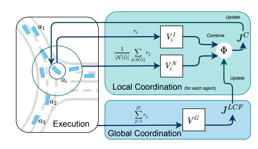
*Fig 1. The framework of CoPO [1]. This is a figure showing the CoPO method framework. CoPO composes by both local and global coordination. In local coordination, the Local Coordination Factor (LCF) is introduced. This factor describes the pereference of the agent, being selfish, competitive or cooperative. This is a common mearsure of social activivity and psychology. Comparing to individual PPO, the introduction of this factor can make the agent take consideration of neibouring agents and achive a better local optimal instead of a sub-optimal policy. So we could observe that as the model shows, the local coordination is the combine of individual value and neiborhood value. The question comes to how to choose this LCF parameter. And this is achieved by global coordination. We try to maximize the global objective with the change of LCF. In this way, the model can update the LCF to be used in the local coordination, as the figure suggests. And finally the policy is updated. The model will deploy 4 neural networks: ploicy network, individual value network, neiborhood value network and global value network. And the whole framework works as the figure suggests. Also, we will train several other MARL methods on same environments to test the CoPO performance. They are IPPO, MFPO and CL. -IPPO: Individual Proximal Policy Optimization. This method will not consider the neiboring agents. In SDP environment, this may lead to sub-optimal results. -MFPO: Mean Field Provimal Policy Optimization. This method take the average states of neighbor agents and take that as imput. We will investigate its performace in later steps. -CL: Curriculum Learning. Curriculum will give different samples different weight depending on their difficulty. Agents will learn gradually.
Environment setting up
MetaDrive is a driving simulator that is compositional, lightweight and realistic. The team considers this driving senario generator a great test generator for the reinforcemnt learning methods.
Following the instructions on MetaDrive website, the team successfully installled MetaDrive and runs a simple driving simulation.
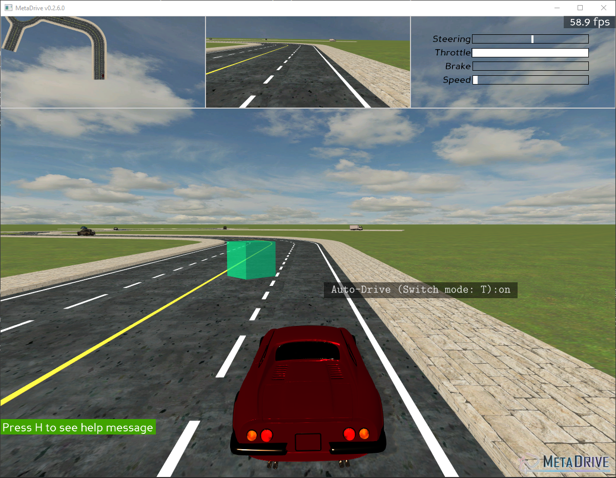
*Fig 2. A test environment of simple driving simulation [2]. For the SDP environment, agent should only have a local observation input to the model. Here we set the observation of each vehicle to: -1.Current state of vehicle, for example: steering, velocity, distance to the side of road -2.Navigation to destination -3.Surrounding information provided by a simulated LiDAR The reward function is given by the longitudinal movement to the destination, along with effect of other parameters.
MARL Environment Example
Metadrive provide us with a few MARL example runs. Here the team practiced on themselves. The example includes different shapes of roads. This different setup could better evaluate the performance of trained model under different circumstances.
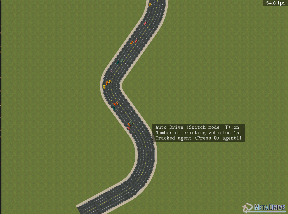
*Fig 3. A MARL enviroment example on a winding road [3].
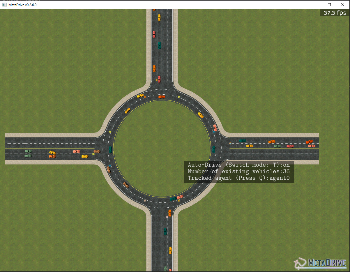
*Fig 4. A MARL enviroment example on a roundaboat [4]. In the examples, the models are already trained and runned. We need further investigation on CoPO.
Model Training
The team tried to train their own model with copo algorithm and other models, following the code provided on Github. In the mid-term report, the team mentioned that they managed to train the model but the evaluation of the model and demonstration is not successful. In later experiment, the team found out the cause of the problem is that there is error in the training progress leading to fails in episodes. I did not understood the program very well and made mistakes when interpreting the results.
The team consider the training faiure is due to certain constraints on my personal computing devices. Though the training process is not successful, thanks to the trained model and checkpoints posted on Github, the team still get to demonstrate the result of the model and do the analysis. The focus will be shifted to analysis the exsisting result and comparison between other algorithms.
With that all being stated, instead of training the whole too big model, we achieved local model training still with the help of the Github guide FAQ. There are several problem encountered in this process. First is that the open_cv package is bugged and need to be moved to a different version. Second is that the platform I used first has an AMD gpu, which indicates no CUDA support anad GPU acceleration. To try to utilize torch GPU acceleration, we moved to a laptop platform with RTX2070, try to train the model locally. However, the algorithm is not as RAM efficient as the CPU method does. And there is barely any improvement comparing to using CPU. The training fails due to RAM overflow.
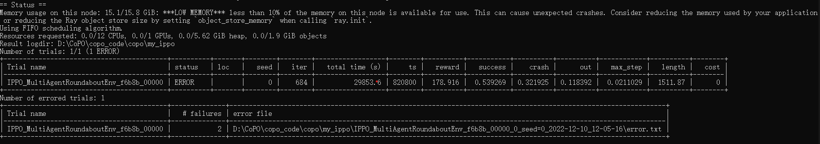
*Fig 5. A failed IPPO train with GPU acceleration [5].
We finally still used CPU train and after 10 hours of training, we successfully trained a model of IPPO locally.
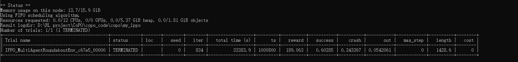
*Fig 6. A IPPO train with CPU [6].
We also plot the result of success_rate vs steps.
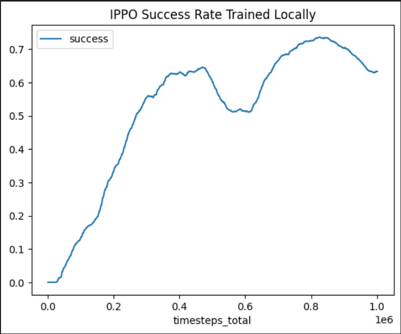
*Fig 7. IPPO train result with CPU [7]. We can see that the trained IPPO model reached 0.7 success rate at best. But we are not going to use this model for evaluation in further steps, as the locally trained models are not as well trained as the well trained ones from Github, thus using those models will lead to a better demonstration of the method and analysis.
Training results
Data from part is evaluated locally with the training data provided. | | Bottleneck | Tollgate | Intersection | Roundabout | Parking Lot | PG Map | |:——————-|:————–|:————–|:—————|:————-|:————–|:————–| | CCPPO (Concat) | 19.55 (15.80) | 3.53 (1.92) | 75.67 (3.18) | 67.82 (4.09) | 12.01 (7.52) | 80.21 (3.58) | | CCPPO (Mean Field) | 14.60 (11.24) | 14.86 (16.47) | 70.79 (6.29) | 71.03 (5.45) | 20.66 (3.47) | 79.56 (3.92) | | CL | 60.60 (22.18) | 37.29 (30.65) | 75.68 (6.24) | 72.28 (5.45) | 21.26 (10.15) | 71.16 (23.69) | | CoPO | 47.39 (19.49) | 27.19 (25.63) | 79.47 (4.97) | 72.82 (6.73) | 19.51 (5.59) | 83.40 (3.13) | | IPPO | 24.04 (18.74) | 4.41 (2.56) | 71.91 (5.27) | 66.43 (4.99) | 16.98 (5.90) | 81.81 (6.50) |
Evaluation on the models
These data are evaluated with data provided from github.
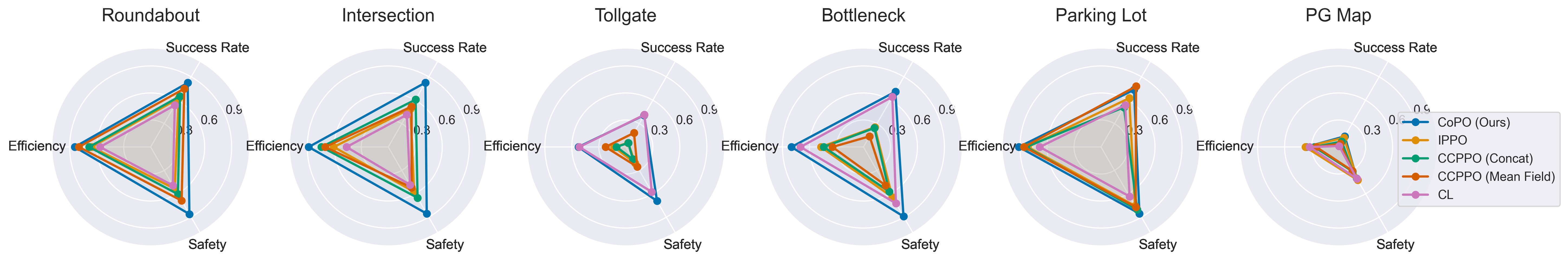
*Fig 8. The evaluation of different methods over different environments [8].
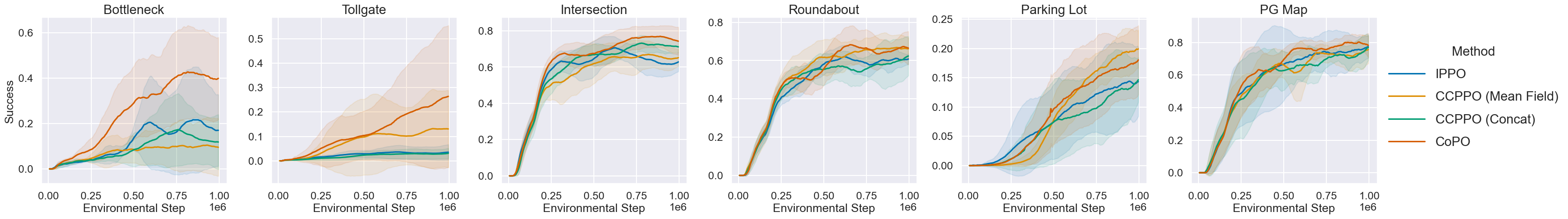
*Fig 9. The success rate vs step of different method in different environments [9].
With the help of the evaluation on the GitHub, I managed to run the evaluation of several policies. Note that the data are from the GitHub, too, as only some of the methods are demonstrated locally.
With the radar plot result, we can see that CoPO has a higher success rate over the other methods. In different environments, CoPO achieved a higher success rate over the others. Also, CoPO also have a higher efficiency and safety value over the other methods, meaning that the vehicles pass at a higher rate and lower crash rate, leading to a better model. Note that some of the algorithm may have a similar success rate in some environment, but the efficiency and safety is much lower than CoPO.
The superior performance of CoPO shows the importance of local and global bi-level coordination.
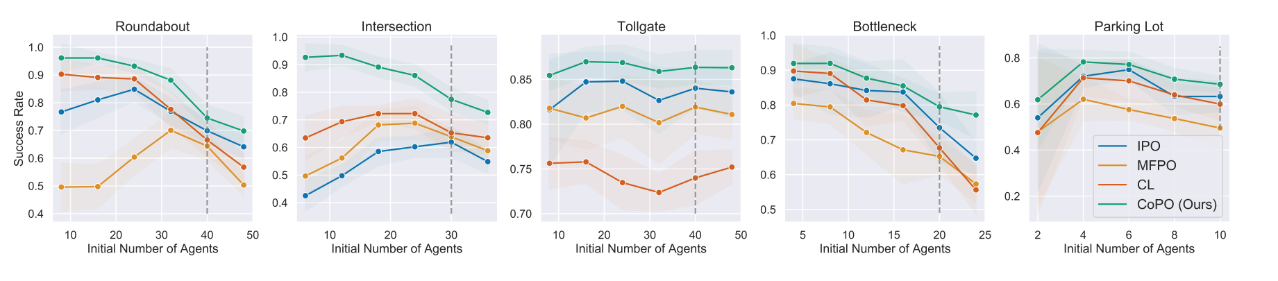
*Fig 10. The success rate vs initial number of agents of different method in different environments [10]. We can also run the trained model under environments with different number of initial agents. As the upper plot from paper suggests, the trained CoPO method have a better performance at any level of agent numbers, further proving the superior performance. We can also observe that for IPO and MFPO, in environment with intensive interactions, like Roundabout and Bottleneck, their performance drops quickly with the increase of the initial number of agents. As the paper suggests, the two models overfit to initial number of agents, while that is not presented in CoPO. In environment Parking Lot, overfitting is presented in all models, which fit our expectation of the paper.
Visualization and Behavior investigation
In this part, we are using the best checkpoints of the trained model provided on the Github. There are may environments you can choose to visualize. Here in the report we will use roundabout, as it is a complicated environment with high density of interaction between agents. The visualization are all locally demonstrated with scripts and metadrive simulator.
Here is a visualization of IPPO trained model.
*Fig 11. The IPPO trained model visulization [11].
We can observe clear congestions and faliures at the start of this model. Agents try to maximize its local reward and dash to the optimal position, while all agents stuck there or hit eachother leading to a low efficiency of passing, as the figure shown below. The success rate is around 0.770. This is relatively good but falirue rate is still not low.
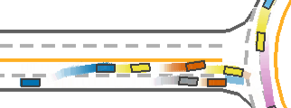
*Fig 12. The IPPO trained model failure case [12].
Here is a visualization of MFPO trained model.
*Fig 13. The MFPO-trained model visulization [13].
We can observe that the performance of Mean field with CF, which is the MFPO method we mentioned before. The success rate is 0.834 which is higher than IPPO, thanks to the measure of taking the average states of neighbors as input. We can still see faliures at beginning, but the whole process is smoother and more efficient. When neighbor agents are sparce or no agents is around, we can see some faliure cases where agents turn around from destination.
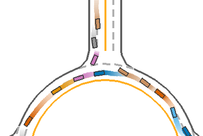
*Fig 12. The MFPO-trained model running case [14].
Here is a visualization of CL-trained model.
*Fig 15. The CL-trained model visulization [15].
We can observe the performance of CL model. We can see some fast agents reaching their objective, while we can also see faliures of agents congesting on the road. Toward the end of simulation, as the number of agents goes down, the efficiency is high and agents reaching their objective at high speed. However, when there are more agents, it seems that the performance is not as good. The average success rate is near 0.783, lower than MFPO.
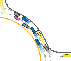
*Fig 16. The CL-trained model congestion [16].
Finally we have the demonstration of CoPO method trained model.
*Fig 17. The CoPO trained-model visulization [17].
We can see a superior performance on CoPO model. This model have a average success rate of 0.86, which is much higher than other models. There are seldom faliure cases in the demonstration. Contributed by the global coordination and LCF tuning, the agent have a similar to real world social decision making process.
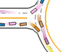
*Fig 18. The COPO trained-model performance at entrance of roundaboat [18]. From the figure above, we can observe that the agents go into the roundaboat in order, where in other models the failures appears the most. The social behavior displayed is complex. The agents cutting, queueing, bypassing and Yielding. They actively switch their preference from cooperative to competitive and back. Unlike other methods, CoPO is more close to real driving logic thanks to LCF factor tuning and better modelling. In this way CoPO achieved high success rate with very low sacrifice of efficiency.
Conclusion and possible improvements
We think CoPO is a very interesting method. Its bi-level coordination of agents is a novel solution to SDP. which is a complicated environment. It is also very interesting to see the strategy trained by CoPO displaying a real-world alike social behavior. It is also meaningful as a new method that could possibly be deployed in real world. Personally, it is a challenge for me to understand the whole algorithm and explore the related methods. But I find it very interesting in the end and I think it is a great start to introduce me to reinforcement learning. There are a lot can be improved in the future. First, we can add not only the trafic flow, we can also add pedestrian crowds simulation to make the senario closer to real world. Second. It is still challenging for vehicles to aquire accurate surrounding data from LiDAR sensors, that cause problems in real-world deploy of the method. Lastly, the test cases are all typical cases generated by metadrive. In the future, real-world maps could be used for more training and performance evaluation.
Thank you for reading! And thanks for all the great works posted and referenced.
Referenced papers
Peng, Zhenghao, et al. “Learning to Simulate Self-Driven Particles System with Coordinated Policy Optimization.” ArXiv.org, 10 Jan. 2022, https://arxiv.org/abs/2110.13827.
Zhang, Kaiqing, et al. “Multi-Agent Reinforcement Learning: A Selective Overview of Theories and Algorithms.” ArXiv.org, 24 Nov. 2019, https://arxiv.org/abs/1911.10635v1.
Hernandez-Leal, Pablo, et al. “A Survey and Critique of Multiagent Deep Reinforcement Learning.” ArXiv.org, 30 Aug. 2019, https://arxiv.org/abs/1810.05587.
Narvekar, Sanmit, et al. “Curriculum learning for reinforcement learning domains: A framework and survey.” arXiv preprint arXiv:2003.04960 (2020).
Rashid, Tabish, et al. “Monotonic Value Function Factorisation for Deep Multi-Agent Reinforcement Learning.” ArXiv.org, 27 Aug. 2020, https://arxiv.org/abs/2003.08839.
Yang, Yaodong, et al. “Mean Field Multi-Agent Reinforcement Learning.” ArXiv.org, 15 Dec. 2020, https://arxiv.org/abs/1802.05438.
de Witt, Christian Schroeder, et al. “Is Independent Learning All You Need in the StarCraft Multi-Agent Challenge?” ArXiv.org, 18 Nov. 2020, https://arxiv.org/abs/2011.09533.
Leibo, Joel Z., et al. “Multi-Agent Reinforcement Learning in Sequential Social Dilemmas.” ArXiv.org, 10 Feb. 2017, https://arxiv.org/abs/1702.03037v1.
Kurach, Karol, et al. “Google Research Football: A Novel Reinforcement Learning Environment.” – ArXiv Vanity, https://www.arxiv-vanity.com/papers/1907.11180/.