Exploring Generalizability in Autonomous Driving Simulation using MetaDrive
One of the most significant challenges in artificial intelligence is that of autonomous vehicle control. The problem is usually modeled as a continuous stream of actions accompanied by feedback from the environment, with the goal of the “agent” being to gradually improve control policies through experience and system feedback via reinforcement learning. A key facet of testing and improving autonomous driving is the use of simulators. Simulators provide an environment to experiment, train and test RL algorithms on benchmarks of success, generalization and safety, without requiring physical resources and environments. This project seeks to understand the functionalities of different autonomous driving simulators, experimenting with multiple algorithms and then moving onto generalization by comparing training on a single generalized environment, and a cascade of environments and determining the optimal configurations that can maximize generalized return.
- Introduction
- Spotlight Video
- Literature Survey and choice of environment
- Methodology and Baseline Experiments
- Experiments - Understanding Generalizaibilty
- Experiments - Extending to MARL
- Conclusion and Future Work
- References
Introduction
In this project, we focus on understanding the various configurations in the MetaDrive environment, and their impact in developing generalizable algorithms towards optimal autonomous driving. The goals of this project can thus be detailed as follows:
- To set up a working autonomous vehicle simulator and successfully initiate training RL based agents.
- To explore the impact of learning under several different algorithms, such as DDPG, TD3 and PPO and develop an agent that can smoothly navigate the environment.
- To extend the above learning towards generalizability along several potential directions, some of which include:-
- Generalizability towards differing map layouts.
- Generalizability of the proposed algorithm and associated parameters across simulator environments.
- Generalizaiblity towards applying the policy in a MARL environment
The code is available here
Spotlight Video
Literature Survey and choice of environment
We performed a comprehensive literature survey on the functionality provided by Metadrive[1] and the types of generalization experiments performed on different autonomous driving environments. MetaDrive is a highly compositional environment where we can generate an infinite number of diverse driving scenarios using procedural generation. This can help us generate a large number of diverse driving scenarios from the elementary road structures and traffic vehicles. It provides us the ability to change lane width, lane numbers and even the reward function. Most generalization experiments in the literature use these parameters to test generalization. One observation is that overfitting happens if the agent is not trained with a sufficiently large training set. Second, the generalization ability can be greatly strengthened if the agents are trained in more environments.
The MetaDrive paper also compares multiple algorithms in their experiments which we try to take into account. We also explored other training environments: SMARTS[2], Duckietown[3], CARLA[4] and SUMMIT[5]. SMARTS (Scalable Multi-Agent RL Training School) is a dedicated simulation platform which supports the training, accumulation, and use of diverse behavior models of road users. The Duckietown environment is also a simulator which allows the training of (Duckiebot) agents in maps customisable with intersections, obstacles and pedestrians. CARLA simulation platform supports flexible specification of sensor suites, environmental conditions, full control of all static and dynamic actors, maps generation and much more. SUMMIT is an open-source simulator with a focus on generating high-fidelity, interactive data for unregulated, dense urban traffic on complex real-world maps.
Our initial investigation involved identifying the ideal environment best suited towards our experimentation. Key considerations include:
- Cross-platform compatibility : The environment should be able to operate on OSX (MacOS with M1/M2 chip) systems / Google Colab without any limitations.
- Lightweight: The environment should provide for observations that allow for rapid training and experimentation , given the project timelines.
- Customizable : Given the extended goal towards exploring generalisability, the chosen environment should allow for some customization of maps, such as layouts, obstacles etc.
Based on the above considerations, we narrowed down on choosing the MetaDrive environment for our experiments and project. MetaDrive is a driving simulator with the following key features:
- Compositional: It supports generating infinite scenes with various road maps and traffic settings for the research of generalizable RL.
- Lightweight: It is easy to install and run. It can run up to 300 FPS on a standard PC.
- Realistic: Accurate physics simulation and multiple sensory input including Lidar, RGB images, top-down semantic map and first-person view images.
We make use of the top-down view for our experiments.
Methodology and Baseline Experiments
Based on our studies from the previous section, we proceed to work towards understanding generalizaibilty on the MetaDrive environment. In this section, we briefly describe the manner in which the experiments were conducted.
For our initial experimentation, we consider the following algorithms: DQN[6], PGD (with baseline)[7], DDPG[8], TD3[9] and PPO[10]. We create a training environment similar to “MetaDrive-Tut-Hard-v0”, with :
- ENVIRONMENT_NUM = 20
- START_SEED = 1000
Each algorithm is trained for a total of 1000000 timesteps (except PPO which we train for 1500000 timesteps) , with differing training hyperparameters based on the algorithm involved.
The figure below provides a comparitive evaluation of each of the algorithms on the same episode. Note that the vehicle in green represents the trained agent.
DQN  |
PGD(with baseline) 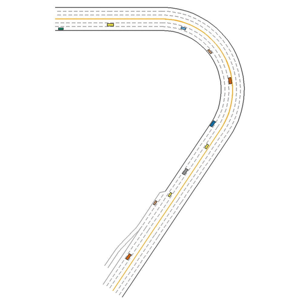 |
DDPG 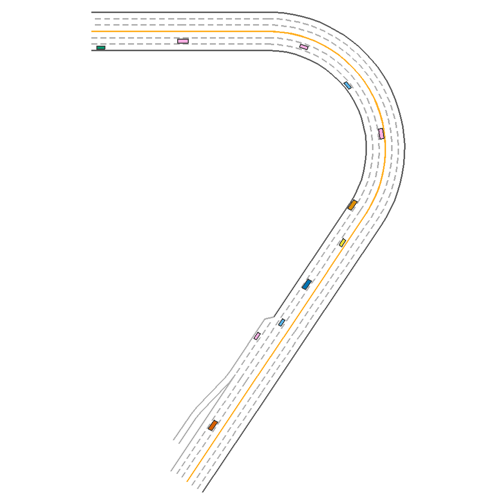 |
TD3 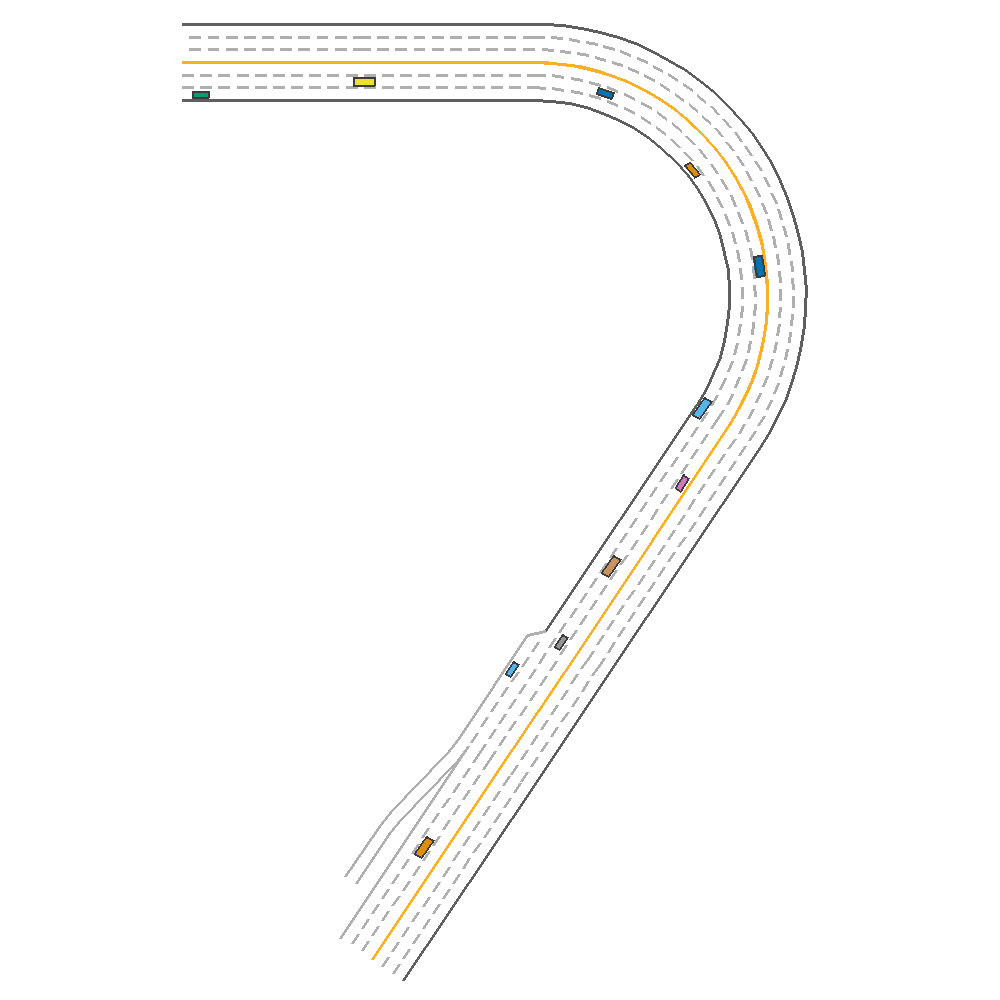 |
PPO 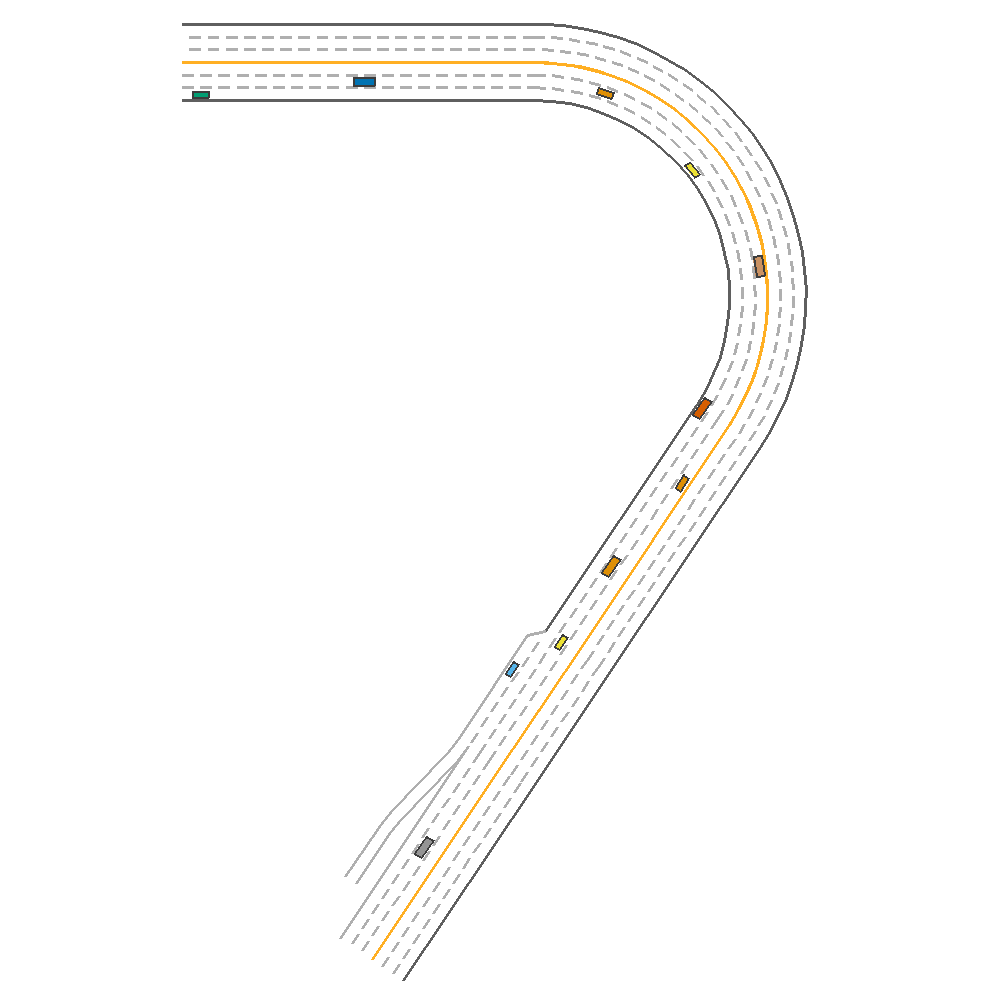 |
Fig 1. Baseline implementation of the various algorithms.
As we can see, we notice promising results from DDPG,TD3 and PPO. We then further evaluate the above trained models on a different episode generated from a modified map configuaration:
- lane_num = 4 (default 3)
- traffic_density = 0.3 (default 0.1)
The figure below demonstraates the results of the above experiments on this unseen map setting.
DQN 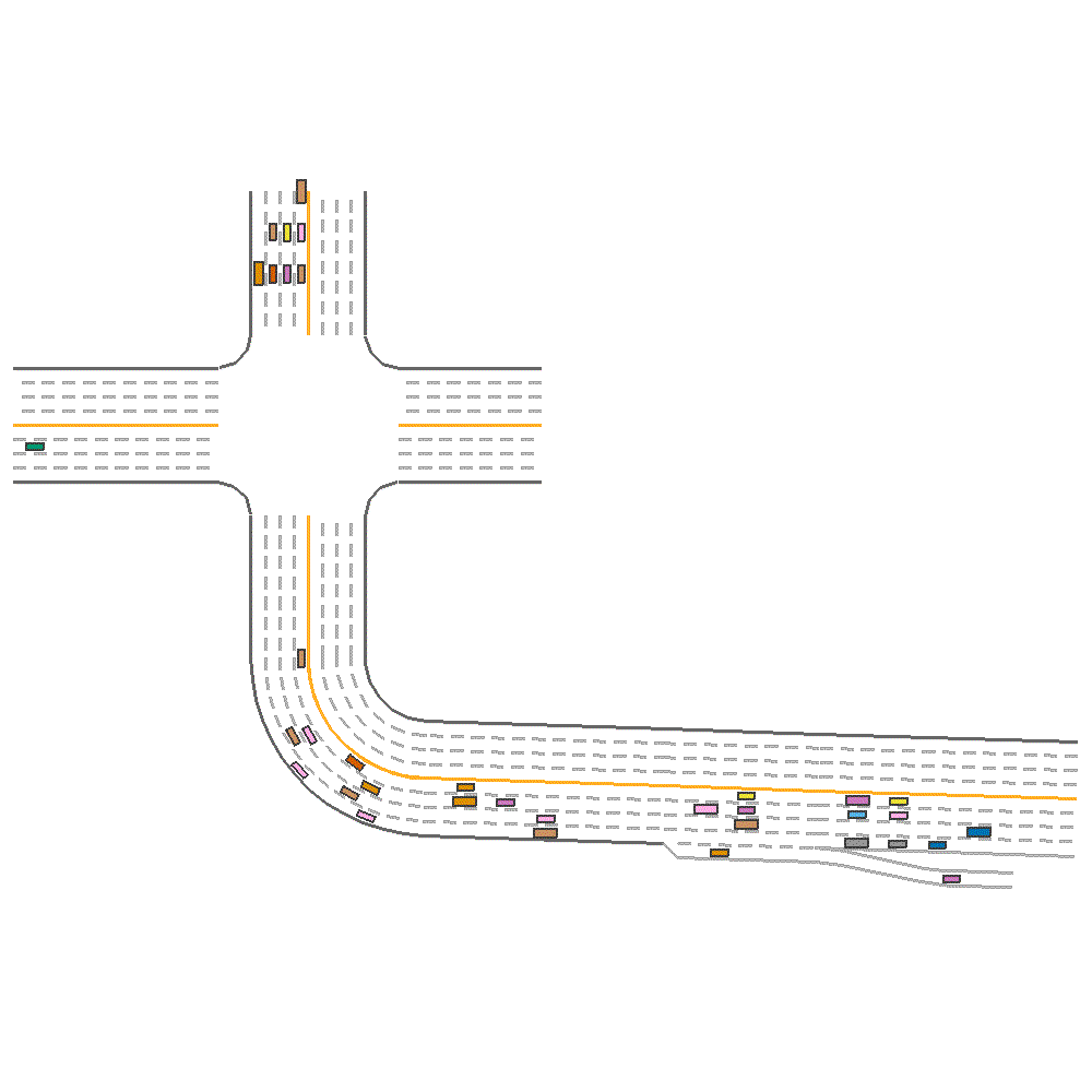 |
PGD(with baseline)  |
DDPG  |
TD3  |
PPO  |
Fig 2. Baseline implementation of the various algorithms on new map configuration.
We also document the baseline quantative results of training the above algorithms in the table below
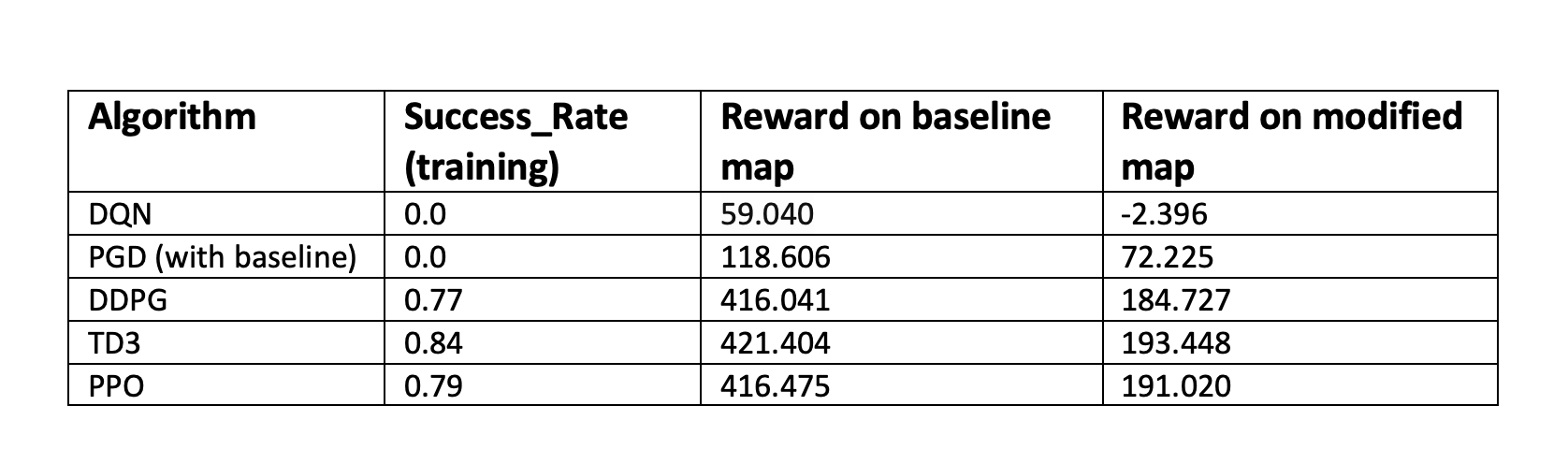 Table 1. Initial Quantitative Analysis.
We choose TD3 as the algorithm of choice for running our experiments moving forward, as it seemed to be most easily configurable, and allowed us to focus more on other configurations and experiments, while giving reasonably high return.
In the following sections, we go through several experiments conducted towards studying generalizaiblity , involving working with different environmental configurations and/or architectural styles.
Experiments - Understanding Generalizaibilty
In this section , we compare and contrast the performance of different configurations to try and understand the contribution of each of the parameters towards generalizability.
Varying Lane number and Width
First, we consider the random_lane_width and random_lane_num to understand their importance and contribution towards performance. We train three different TD3 agents, 2 of which are trained on evnironments with one of the three of random_lane_width and random_lane_num set to true, while the third is trained in an environment where all the parameters are set to True.
Random Lane Num only(reward=123.012)  |
Random Lane Width only(reward=69.10) 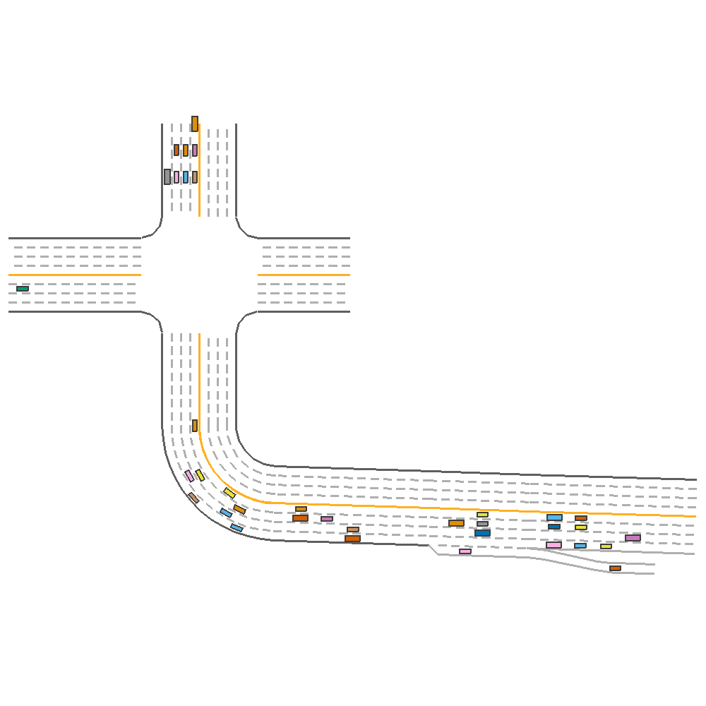 |
Combined(reward=339.44)  |
Fig 3. Effect of Varying Lane Number, Lane Width and both together.
The average reward for each of the agents across 10 test environments are documented below
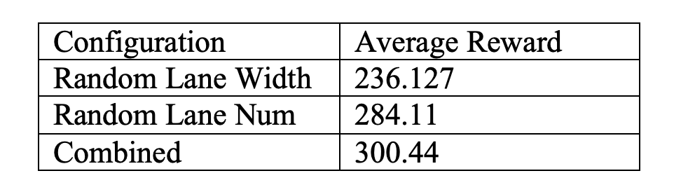 Table 2. Quantitative Analysis for Lane Number, Lane Width.
From the above figure, we can observe that both parameters are critical towards training a generalziable model.
Modifying the Reward Function
Next , we consider the impact of the two reward parameters: driving_reward and speed_reward. We consider two experiments, as shown in Figure 4 below.
Driving Reward=5, Speed Reward=0.1(reward=336.85) 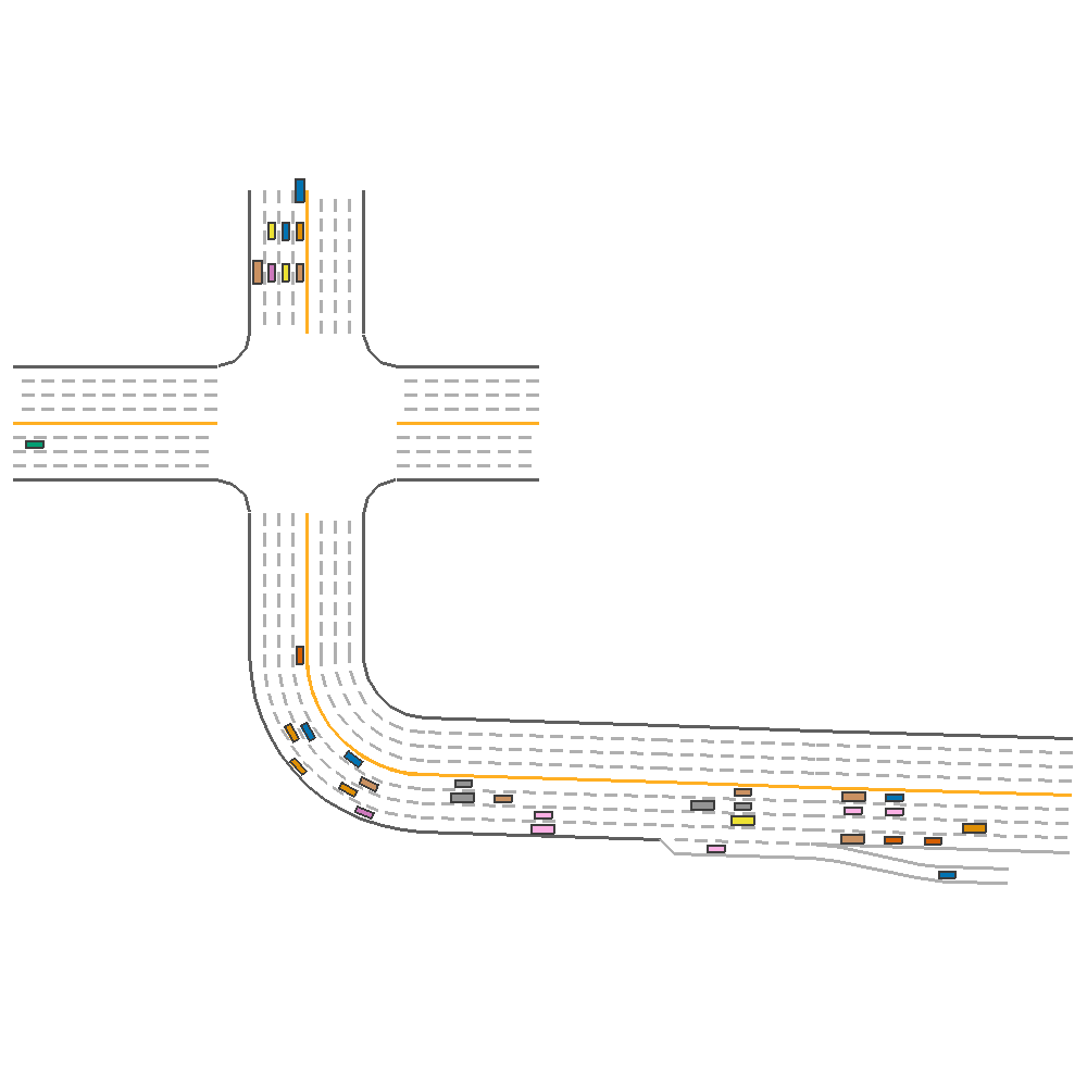 |
Driving Reward=0.5, Speed Reward=0.5(reward=122.89)  |
Fig 4. Effect of Varying Reward coefficients.
The average reward for each of the agents across 10 test environments are documented below
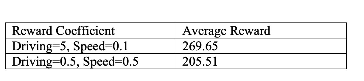 Table 3. Quantitative Analysis for Reward coefficients.
From the above figure, we can observe that having a good driving reward is more crucial than speed reward towards generating a more sustainable agent, as a high speed reward can cause the agent to crash.
Working with different neural network architectures
In this section, we move away from environmental configurations, and focus on the neural network associated with the TD3 Actor and Critic. Each of the agents are trained on a Generalization-friendly environment, where random_lane_num , random_lane_width and random_traffic are all set to True. In this section, rather than focusing on the direct performance on a training environment, we look at the training curves and observe the trends and results to see if any configurations could provide more stable training.
First, we try to vary the network architecture by using a Convolutional Network. Since the observation is a Lidar observation that’s of dimension (batch_size, state_dim), we use Conv1d layers. Figure 5 shows the training curves when attempting to use 1D Convolutions for both the actor and critic.
Original TD3 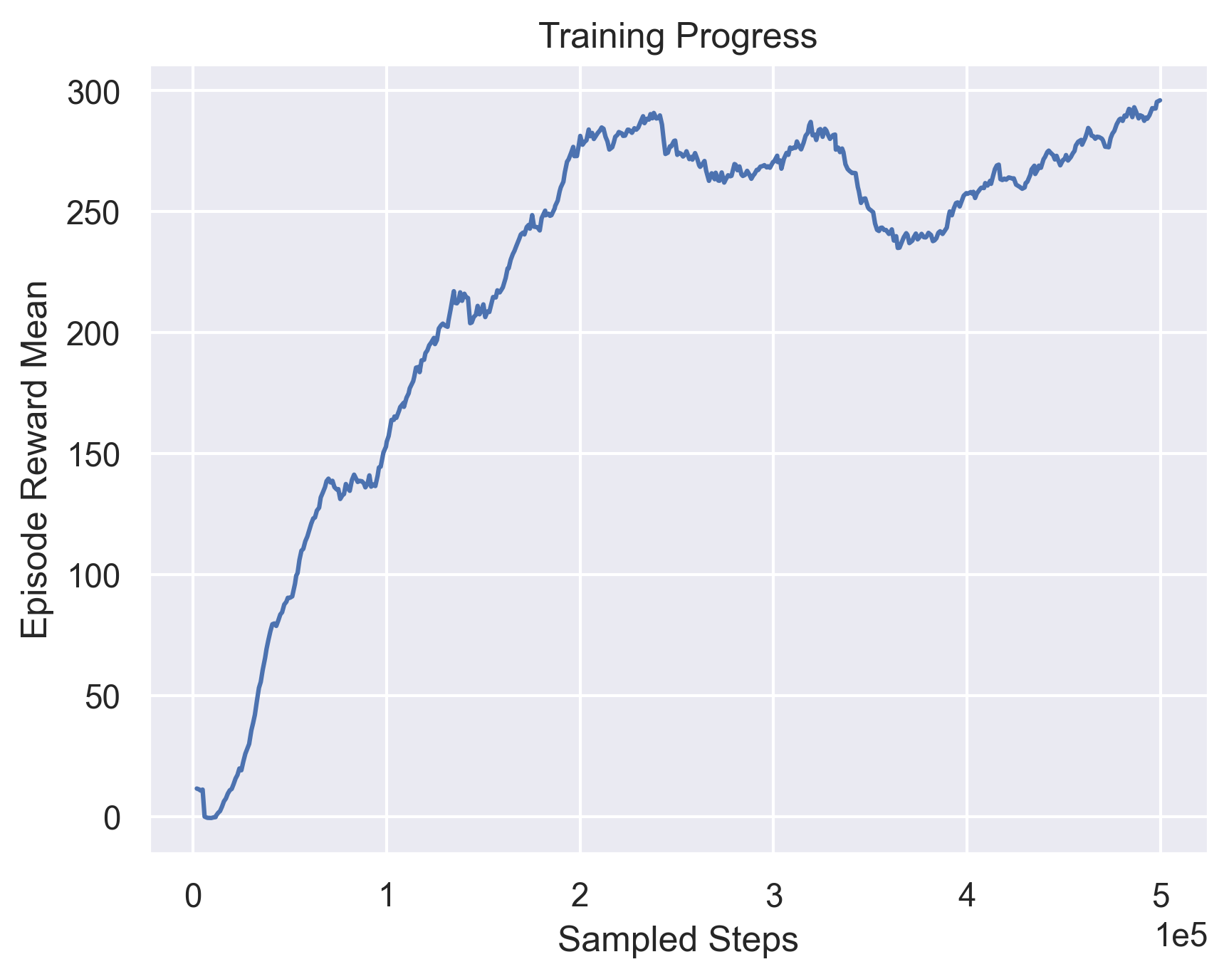 |
TD3 with 1dConv in Actor 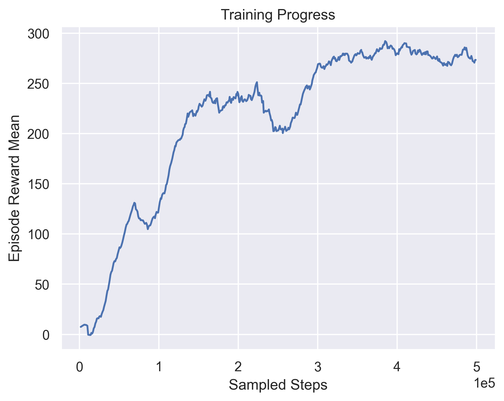 |
TD3 with 1dConv in Critic 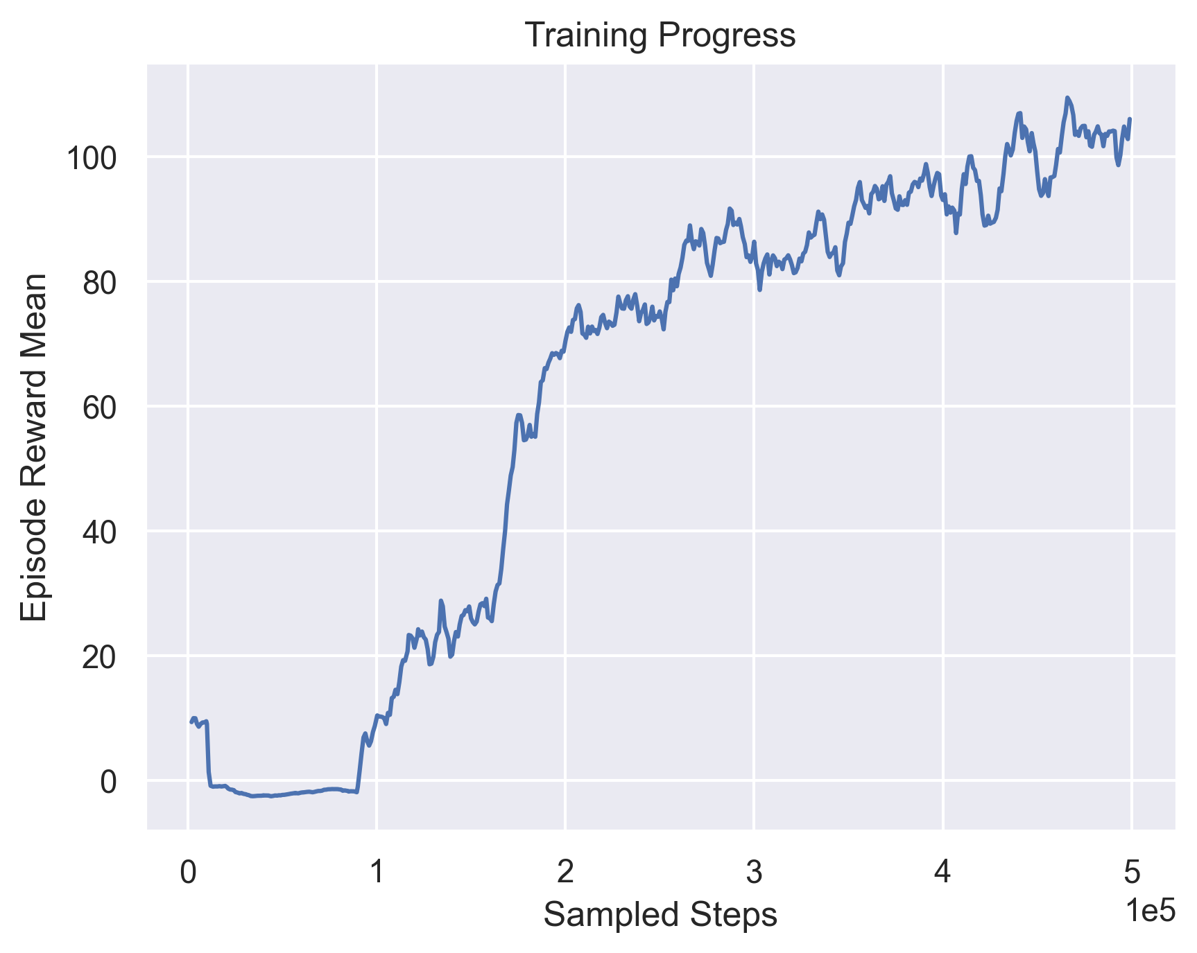 |
Fig 5. Using 1D Convolutions.
As we can see, convolutional layers do not provide any positive impact towards improving training performance. In fact, trying to set the critic layers to Conv1d layers severely degrades performance. This can be accounted to the inherent observation structure and the inabilty of 1D Convolutions to extract anything extra meaningful from these observations.
Next, we focus on trying to manipulate the optimizers and the non-linear activations. We try to use AdamW[11] optimizer instead of Adam since it has a better weight decay policy that is stated to improve generalization in general deep learning. We also consider the effect of using Leaky Relu[12] as a non-linear activation instead of Relu. The effect of these experiments is shown in Figure 6.
| Original TD3 |
AdamW optimizer 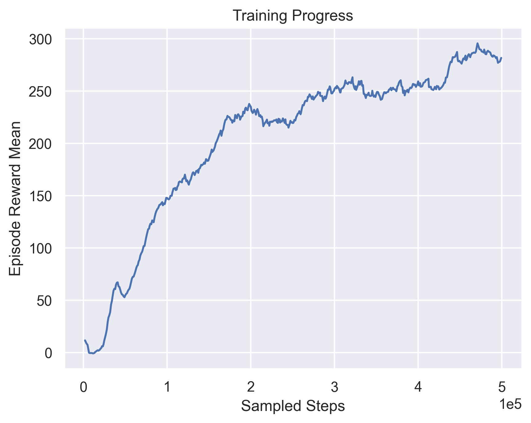 |
Leaky Relu 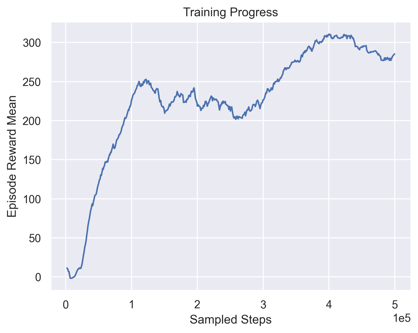 |
Fig 6. Modifying the optimizer and non-linear activation function.
Again, we don’t observe any immediate impact in the training performance, apart from a slight boost in the performance obtained by Leaky ReLU. However, we observe that the training curves are more stable in the case of AdamW and Leaky ReLU as opposed to the base case, with no major sharp dips in performance. Thus, we consider these configurations in our next experiments as well.
Experiments - Extending to MARL
We next focus on extending our experiments to MARL. Specifically, we attempt to see whether we can train an agent in Single Agent environments based of MetaDriveEnv and SafeMetaDriveEnv , and attempt to deploy multiple agents in a Multi-Agent RL environment , each of which use the single agent policy.
Environment chaining
We first attempt to perform a trick of environment chaining, where we attempt to try and train an agent for fewer epochs over multiple environments, transferring the knowledge from one environment to another. Initially, we try to train an agent across three different general MetaDrive environments, each with varying parameters. As shown in Figure 7 however, simply directly trying to chain environments without any logical pattern severely impacts performance.
Original TD3(reward=790.81)  |
Chained MARL agent(reward=164.37) 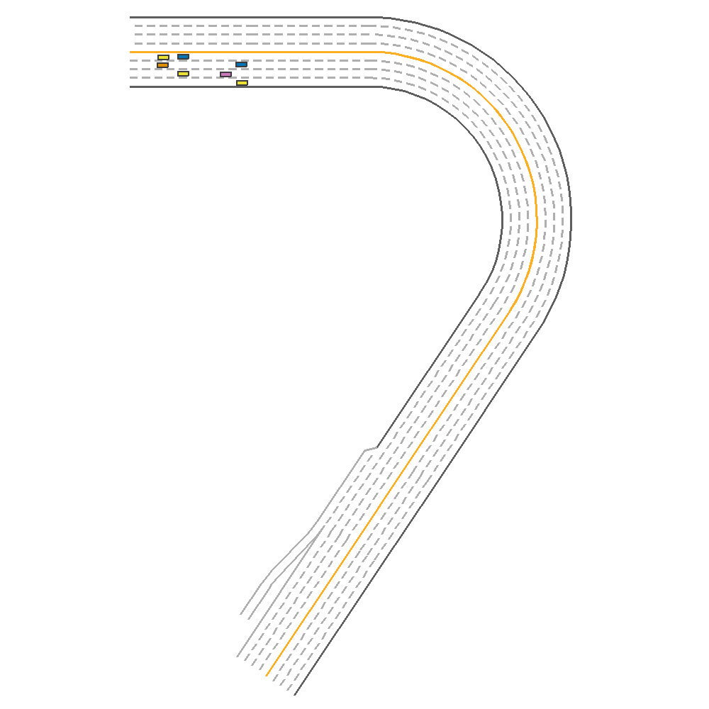 |
Fig 7. Effect of just randomly trying to chain environments. The “Original TD3” agent in the above case is the same agent as presented in Figure 3 (trained on a single environment with all 3 configurations set to random).
Chaining with safe environements
We next carefully try to construct a chaining sequence, focusing on different aspects. In particular, given the need for safety to ensure individual agents can drive properly, we attempt to include SafeMetaDriveEnv into the chaining sequence. We end up with the below environment sequence:
- First environment is a SafeMetaDriveEnv with focus on driving reward and lateral reward to ensure the agent learns safe driving early (driving_reward=1.3, use_lateral_reward=0.5)
- The second environment is a general high-traffic environment (traffic_density=0.3)
- The third environment is another Safe Driving environment with a focus on speed (speed_reward=0.4)
Figure 8 shows the results of chaining on the above configurations. As we can see, the above chanining experiment produces a much better result, near comparable with the original single environment setting.
| Original TD3(reward=790.81) |
Safe Chained MARL agent(reward=744.5)  |
Fig 8. Effect of chaining with a safe environment.
Final construct - chained environment + best policy compared to original work
Finally, in order to further boost performance, we use the above environment chaining but make certain changes to the TD3 training algorithm to attempt to boost performance.
- We make use of the AdamW optimizer and Leaky ReLU activation functions to stabilise training.
- We consider the noise that is added to the “next action” to calculate the Q targets. In order to stabilise the impact of noise, we gradually reduce it and cycle the standard deviation of the noise as the agent is trained across environments (starting as policy_noise -0.3 and reducing it to 0 over time). The idea behind this cyclic decrease is that as the agent is further trained, we allow the Q_targets to be directly computed off the actor’s lerned behaviour, rather than relying on noise.
- We also make a small change to how the Q_target is obtained. Instead of just taking the minimum of Q1 and Q2, we add a small term to this, namely: Q_intermediate = torch.min(Q1,Q2) + 0.01*(torch.max(Q1,Q2)-torch.min(Q1,Q2)). The idea being to try and push the loss towards bringing Q1 and Q2 together, ensuring a more stable actor policy is learned.
With the above configurations we train a new agent, and observe that it beats our original trained single environment agent quite comfortably in performance, as shown in Figure 9.
| Original TD3(reward=790.81) |
New Chained MARL agent(reward=1422.21)  |
Fig 9. Effect of chaining with a safe environment and modified configurations.
Table 4 shows a comparison of all the 4 approaches towards MARL generalizaiblity when tested on 10 different test environments.
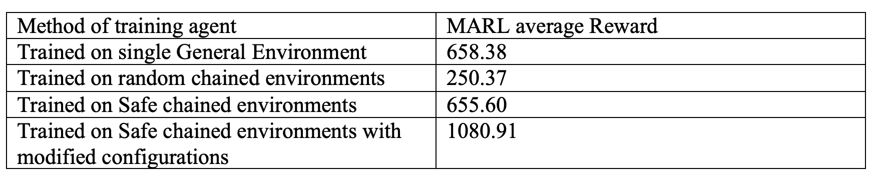 Table 4. Quantitative Analysis for methods towards geneeralizable MARL agent.
Num of agents in MARL
As an ablation study, we also show the degradation in performance of the agent as we increase the number of agents.
5 agents(reward=657.87) 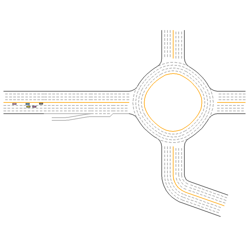 |
15 agents(reward=350.86) 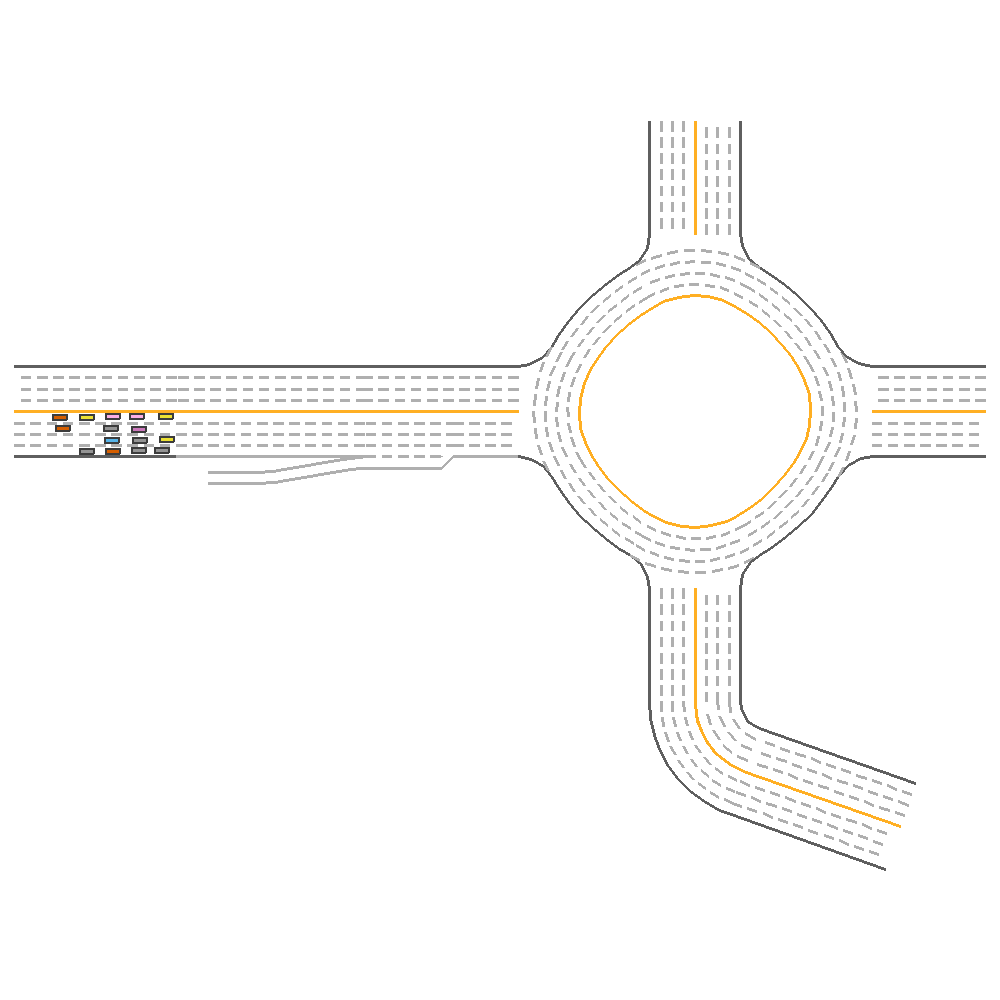 |
25 agentsreward=(327.14)  |
Fig 10. Effect of number of agents.
Conclusion and Future Work
This project sought to explore the potential for generalizabilty in the MetaDrive environment, with a focus on several aspects such as modifying environmental configurations and agent configurations. We then also attempt to observe how these agents trained on single agent environments can generalise to working on MARL environments, without including an MARL agent in the loop. As we observe, as a consequence of all our experiments, we are able to train a strong agent in the MARL settings using agents trained in a creative manner in the Single Agent setting. Future work can include further studying the neural network architecture and loss functions associate with TD3, with a goal of delivering an even more stable generalizable agent.
References
[1]Li, Quanyi, et al. “Metadrive: Composing diverse driving scenarios for generalizable reinforcement learning.” IEEE transactions on pattern analysis and machine intelligence (2022).
[2]Paull, Liam, et al. “Duckietown: an open, inexpensive and flexible platform for autonomy education and research.” 2017 IEEE International Conference on Robotics and Automation (ICRA). IEEE, 2017.
[3]Zhou, Ming, et al. “Smarts: Scalable multi-agent reinforcement learning training school for autonomous driving.” arXiv preprint arXiv:2010.09776 (2020).
[4]Dosovitskiy, Alexey, et al. “CARLA: An open urban driving simulator.” Conference on robot learning. PMLR, 2017.
[5]Cai, Panpan, et al. “Summit: A simulator for urban driving in massive mixed traffic.” 2020 IEEE International Conference on Robotics and Automation (ICRA). IEEE, 2020.
[6]Mnih, Volodymyr, et al. “Playing atari with deep reinforcement learning.” arXiv preprint arXiv:1312.5602 (2013).
[7]Sutton, Richard S., et al. “Policy gradient methods for reinforcement learning with function approximation.” Advances in neural information processing systems 12 (1999).
[8]Lillicrap, Timothy P., et al. “Continuous control with deep reinforcement learning.” arXiv preprint arXiv:1509.02971 (2015).
[9]Fujimoto, Scott, Herke Hoof, and David Meger. “Addressing function approximation error in actor-critic methods.” International conference on machine learning. PMLR, 2018.
[10]Schulman, John, et al. “Proximal policy optimization algorithms.” arXiv preprint arXiv:1707.06347 (2017).
[11]Maas, Andrew L., Awni Y. Hannun, and Andrew Y. Ng. “Rectifier nonlinearities improve neural network acoustic models.” Proc. icml. Vol. 30. No. 1. 2013.
[12]Kingma, Diederik P., and Jimmy Ba. “Adam: A method for stochastic optimization.” arXiv preprint arXiv:1412.6980 (2014).