Ensemble RL - Apply Ensemble Methods on Reinforcement Models using MetaDrive
Ensemble method helps improve models’ performance by combining multiple models instead of using a single model. These methods are wildly used in many Machine Learning tasks. However, there is not much implementation in the Reinforcement Learning area. In this project, we will apply ensemble methods in Reinforcement Learning to our autonomous driving task based on the MetaDrive platform. We trained Proximal Policy Optimization (PPO), Twin Delayed DDPG (TD3), Generative Adversarial Imitation Learning (GAIL), and Soft Actor-Critic (SAC) models as baseline models. We investigated different ensemble methods based on these models. The overall result for the model after the ensemble is slightly better than the ones without the ensemble, but in some cases, we gain much better results.
- 1 Introduction
- 2 Related Works
- 3 Base Model Performance
- 4 Methodology and Experiments
- 5 Conclusion and Future Works
- 6 Video Demo
- 7 References
1 Introduction
Recently, Reinforcement learning has been wildly used in autonomous driving and the driving task has high complexity, and is hard to construct a safe model or policy. Nowadays many different methods are developed and used in reinforcement learning, such as Proximal Policy Optimization (PPO)[1], Twin Delayed DDPG (TD3)[2], Generative Adversarial Imitation Learning (GAIL)[3], and Soft Actor-Critic (SAC)[4], to name a few. These models achieve pretty impressive results on autonomous driving tasks so far by themselves but currently no published effort tried to improve performance by combining these models. In this project, we investigate different ways of combining these methods and checked if there are improvements.
One popular method that could easily combine different models is the ensemble method. Ensemble methods[5] are techniques that aim at improving the accuracy of results in models by combining multiple models instead of using a single model. These are wildly used machine learning problems such as classification and improving the accuracy by taking a (weighted) vote of their predictions. There are also ensemble methods such as bagging and boosting.
In this project, we investigated whether applying ensemble methods to reinforcement learning algorithms in autonomous driving tasks will improve rewards and performance. We investigated several different ways to ensemble different models. We trained and tested the following several ensemble methods: (1) Ensemble by taking a (weighted) vote of their predictions. (2) Ensemble by using a human-defined strategy of predictions. (3) Learning the weight of different models using reinforcement learning and ensemble by taking a (weighted) vote of their predictions. The overall result for the model after the ensemble is slightly better than the ones without the ensemble, but in some cases, we gain much better results.
The paper is organized as follows. Section 2 summarized all the related works in reinforcement learning, autonomous driving simulation platforms, and ensemble methods. Section 3 showed the basedline models and their performance. Section 4 illustrated all our methods in detail and presented the experiment settings and experiment results. Section 5 demonstrated our conclusion. And we briefly talked about our future works in section 6.
2 Related Works
2.1 Platform
There are a variety of simulation platforms for training reinforcement learning agents for self-driving vehicles. The Team started with CARLA[6], as that is the most popular platform for these simulations, but we have moved away from this simulator because we do not have machines that supports its environment. Therefore, the Team instead used Metadrive[7], a more light-weight simulator that still provides realistic simulations. There are also simulators such as Nocturne[8], SMARTS[9], AirSim[10], each designed to focused on specific aspect of driving.
2.2 SOTA Reinforcement Learning Models
In the project, we have experimented with a number of Reinforcement learning and Imitiation learning models. Proximal Policy Optimization (PPO)[1] is a policy gradient method that constrained policy update size by adding KL penalty, allowing for ease of tuning and good sample efficiency with relatively simple approach compared to ACKTR and TRPO. Twin Delayed DDPG (TD3)[2] is a Q-learning model that uses Clipped Double-Q Learning, Delayed policy update and Target Policy smoothing addresses the issue of of Q-function inaccuracy in DDPG and other DQN algorithms. Generative Adversarial Imitation Learning (GAIL)[3] is an imitation learning approach that uses a discriminator network as adversary to imitate the given expert. Soft Actor-Critic (SAC)[4] is a Off-policy Actor-critic algorihm that based on the maximum entropy reinforcement learning framework, by combining Q-learning methods with trust region techniques in policy gradient methods. There are also modification of these algorithms or their predecessor for Distributed RLs, such as A2C, A3C, Apex. There are also derivative free approaches such as Evolution Strategies and Augmented Random Searches, and also Model RL approaches such as Dreamer(Image only) and Model-Based Meta-Policy-Optimization(MB-MPO). These algorithms can be found with RLLib’s implementations [11].
2.3 Ensemble Methods
Ensemble method combines multiple simplier models in obtain a better model for the tasks. Ensemble Methods are well studied in Machine Learning, with many methods proposed, as shown in the survey[12]. These approaches includes Bagging, Random Forest, Rotation Forest. Boosting methods like AdaBoost are not considered as it has dependence between the model (training subsequent model base on error sample from previous). There are also Meta-learning methods like stacking.
Ensemble methods in RL is also being researched, with a variety of methods to combine actions being researched by Wiering and van Hasselt[13]. These method includes Majority Voting, Rank Voting, Boltzmann mult and Boltzmann add. There are also frameworks being proposed, like SUNRISE[14]. However, they are only using human-tuned techniques for combining actions, but not meta-learning approaches.
3 Base Model Performance
| Models | Episodic Reward |
|---|---|
| PPO | 194.027 |
| TD3 | 340.056 |
| GAIL | 269.660 |
| SAC | 273.224 |
Table 1. Base Model Performance.
4 Methodology and Experiments
In this section, we will investigate different ways of ensembling several pretrained models. We mainly tried the following three different ways to ensemble models. (1) Ensemble by taking a (weighted) vote of their predictions. (2) Ensemble by using a human-defined strategy of predictions. (3) Ensemble using reinforcement learning.
4.1 Naive Average with Weight
The first ensemble method we use is taking a weighted vote of baseline models’ predicted actions. The predicted action after the ensemble is calculated using the following equation
\(a=\sum_i w_i a_i\), subject to \(\sum_i w_i = 1\)
where \(a_i\) is the prediction action from the \(i\)-th model and \(w_i\) is a hyperparamter representing the weight for each parameter. We also make sure the sum of all weights is equal to 1.
In this method, during the prediction phase, when we get an observation from the environment, we pass the observation to the baseline models and collect predicted actions from them. The final action we use is the weighted average of the collected actions.
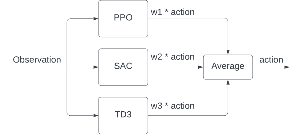
Fig 1. Ensemble by Naive Average with Weight.
4.1.1 Experiment Result and Visualization
We experiment with the methods with different combinations of baseline models trained on MetaDrive Environment and evaluate the model on 10 complicated environments using MetaDrive. The combinations and testing results we tested are shown in the table below.
| Models | Weight | Episodic Reward |
|---|---|---|
| PPO, GAIL | 1:1 | 216.536 |
| PPO, TD3 | 1:1 | 298.235 |
| PPO, TD3, GAIL | 1:1:1 | 279.224 |
| TD3, PPO, SAC | 1:1:1 | 324.545 |
| TD3, PPO, SAC | 2:1:2 | 343.507 |
| TD3, PPO, SAC | 2:2:1 | 322.389 |
| TD3, PPO, SAC | 1:2:2 | 315.341 |
| TD3, PPO, SAC | 3:1:1 | 370.225 |
| TD3, PPO, GAIL | 1:1:8 | 268.913 |
| TD3, PPO, GAIL | 8:1:1 | 231.019 |
Table 2. Experiment Result for Ensemble by Naive Average with Weight.
Based on table 2, compare to a single model performance (baseline performance) shown in table one, we found that, in most cases, the ensembled reward is better than the worst baseline it used and worst than the best baseline models it used. In some cases, the reward of the ensembled model is better than all the models it used.
We also visualized the prediction with the best ensembled model (TD3, PPO, SAC, 3:1:1) on one of our selected environments as below.
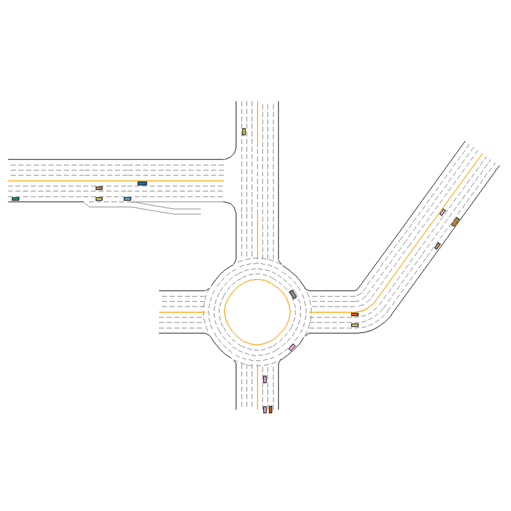
Fig 2. Ensemble with Human-Defined Strategy.
4.2 Ensemble with Human-Defined Strategy
The first method, Naive Average with Weight, couldn’t increase the performance significantly. We believe one possible problem for it might be averaging might leads to actions doesn’t make sense. Consider the following scenario (Fig. 3). Suppose we want to pass over the gray car in front of our green agent. Model 1 suggests we turn left and accelerate. Model 2 suggests we turn right and accelerate. If we average these two actions the ensembled action will be going straight and accelerating, in which case we will just hit the grey car in front of us.
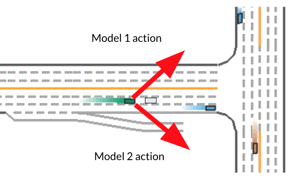
Fig 3. Problematic Senario using Ensemble by Naive Average with Weight.
To avoid this situation from happening, we construct the following strategy (Fig. 4). Using the strategy, during the prediction phase, when we get an observation from the environment, we pass the observation to the baseline models and collect predicted actions from them. We then do a majority vote on the directions, then the final ensembled action should be the average of the actions with the majority actions.
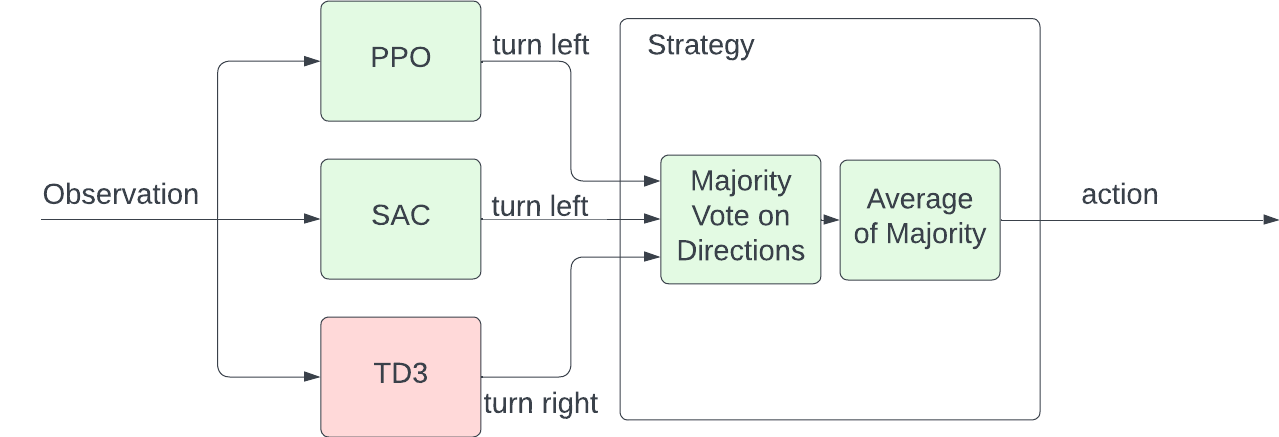
Fig 4. Ensemble with Human-Defined Strategy.
The final action is calculated by
\[\textit{major_direction} = \textit{majority} (sign(a_i[0]))\]Take Fig. 4 as an example, suppose we have three models, PPO, SAC, and TD3 model. PPO, SAC predicts turning left. TD3 Predicts turning right. Then the majority directions will be turning left. Thus the final action we take will be the average of action of PPO and SAC.
4.2.1 Experiment Result and Visualization
We experiment with the methods with 2 combinations of baseline models trained on MetaDrive Environment and evaluate the model on 10 complicated environments using MetaDrive. The combinations and testing results we tested are shown in the table below.
| Models | Episodic Reward |
|---|---|
| TD3, PPO, SAC | 363.580 |
| PPO, TD3, GAIL | 268.913 |
Table 3. Experiment Result for Ensemble with Human-Defined Strategy.
Based on Table 3, compared with the baseline model performance in Table 1, and naive average with weight method performance in Table 2. We found that the performance is pretty close to the performance of naive average with weight method. For TD3, PPO, SAC combination, we have reward 363.580 on our test environments, which is better than 324.545 using naive average with weight method. While for PPO, TD3, GAIL combination we have reward 268.913, which is slightly worse than 279.224 using naive average with weight method.
We also visualized the prediction with the best ensembled model (TD3, PPO, SAC) on one of our selected environments as below.
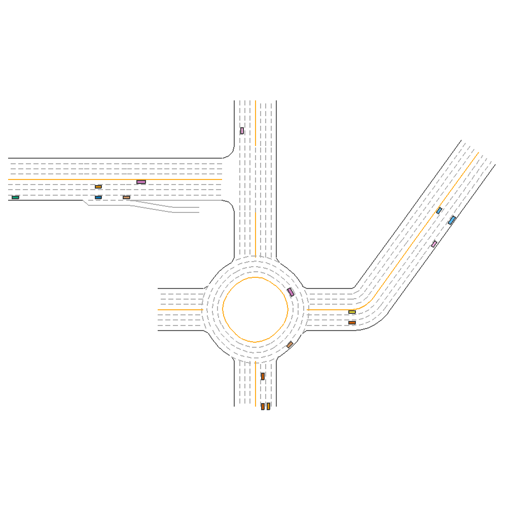
Fig 5. Ensemble with Human-Defined Strategy.
4.3 Learned Ensemble using Reinforcement Learning
In section 4.1 and 4.2, we introduced two ensemble methods that utilize the baseline model only in the prediction phase. And the way to combine these models are settled. eg. the weight for different models are hyperparameters and remains constant for all observations.
In this section, we purpose a new way to ensemble these baseline models using a new reinforcement learning model. We train a new RL model called selection model that able to select the best baseline model given the current observation. The detailed structure is demonstrated in Fig. 6.
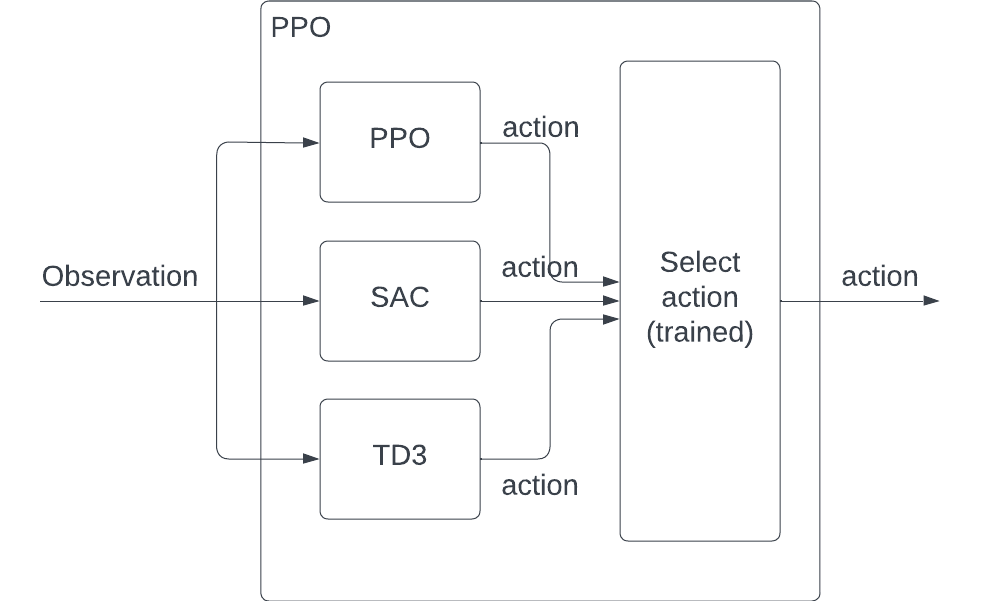
Fig 6. Ensemble using Reinforcement Learning.
In our following experiment, we trained several PPO models as our selection models that are able to select the best action from the baseline models. The action for our selection model is the weight we assigned to different baseline models. Given an observation, we will first pass this observation to the baseline models to generate the baseline actions. We will also pass the observation to our selection model and produce one selection action. The final action provide to the MetaDrive environments will be calculated as below.
\[a_{final} = \sum_{i=0}^N a_{select}[i] \times a_i\]for \(N\) baseline models, where \(a_{select}[i]\) is the weight for the \(i\)-th model we get from our selection model based on observation. \(a_i\) is the action produced by baseline model \(i\) based on observation.
In the following 3 sections, we trained 3 different selection models based on different baseline models.
4.3.1 Ensemble Different Models
The first group of baseline models we choose are the PPO, TD3, and SAC model described in section 3. After training, we found our best training reward is around 350. And evaluation reward is 297.975.
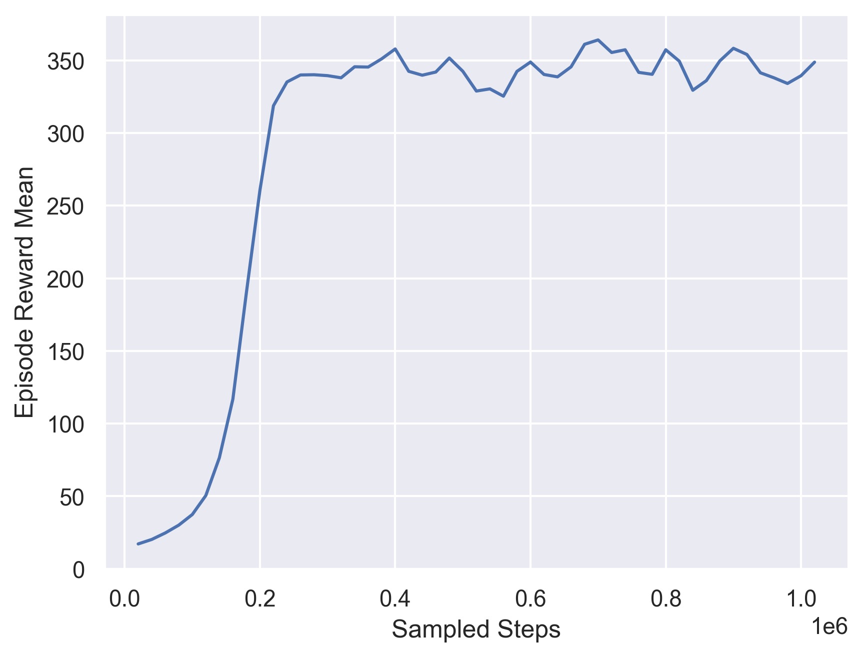
Fig 7. Training Curve for Ensemble PPO, TD3, and SAC model.
Also notice from the training curve, we found that we are able to achieve very high reward in very few iteration.
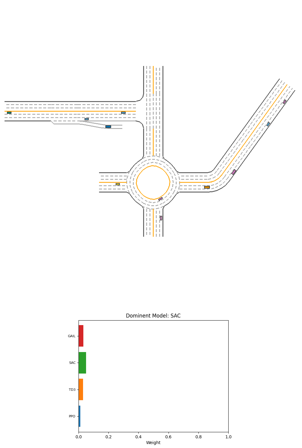
Fig 8. Evaluation Result for PPO Ensemble Model.
We also visualize the weight for each model on one of our evaluation environments and find that if the baseline model able to achieve higher reward, the ensembled model are more likely to select it. eg. we seldom see PPO baseline model have a very high weight.
4.3.2 Ensemble Different PPO Models Trained on Different Senarios
Besides let our selection model to select on models trained on different methods. We also tried train models with different specializations. In this section, we trained 3 modeled using PPO, and each model are focusing on one specific senarios.
The first model we trained as baseline is a PPO model trained on environment that only contains straight road. The training curve for this model is showed below and the evaluation episodic reward is 87.356.
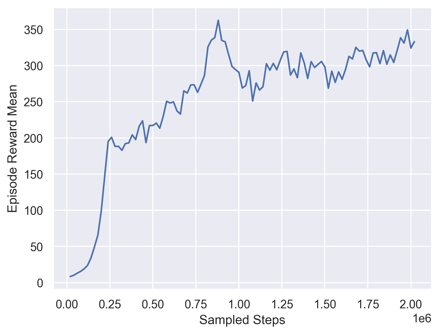
Fig 9. Evaluation Result for PPO Ensemble Model.
The second model we trained as baseline is a PPO model trained on environment that only contains intersections. The training curve for this model is showed below and the evaluation episodic reward is 143.737.
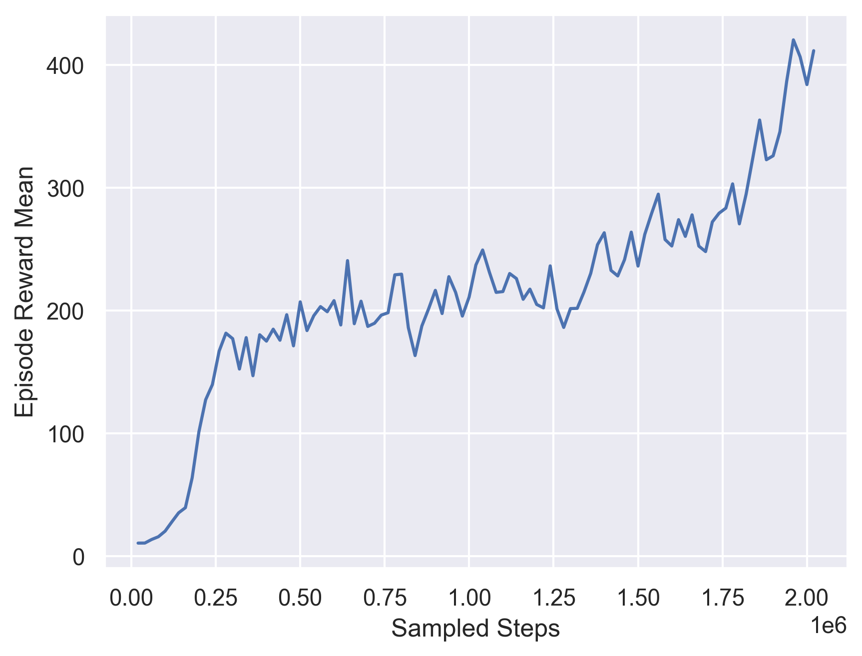
Fig 10. Training Curve for a PPO on Intersection Road Environments.
The third model we trained as baseline is a PPO model trained on environment that only contains Circular and Roundabouts. The training curve for this model is showed below and the evaluation episodic reward is 216.100.
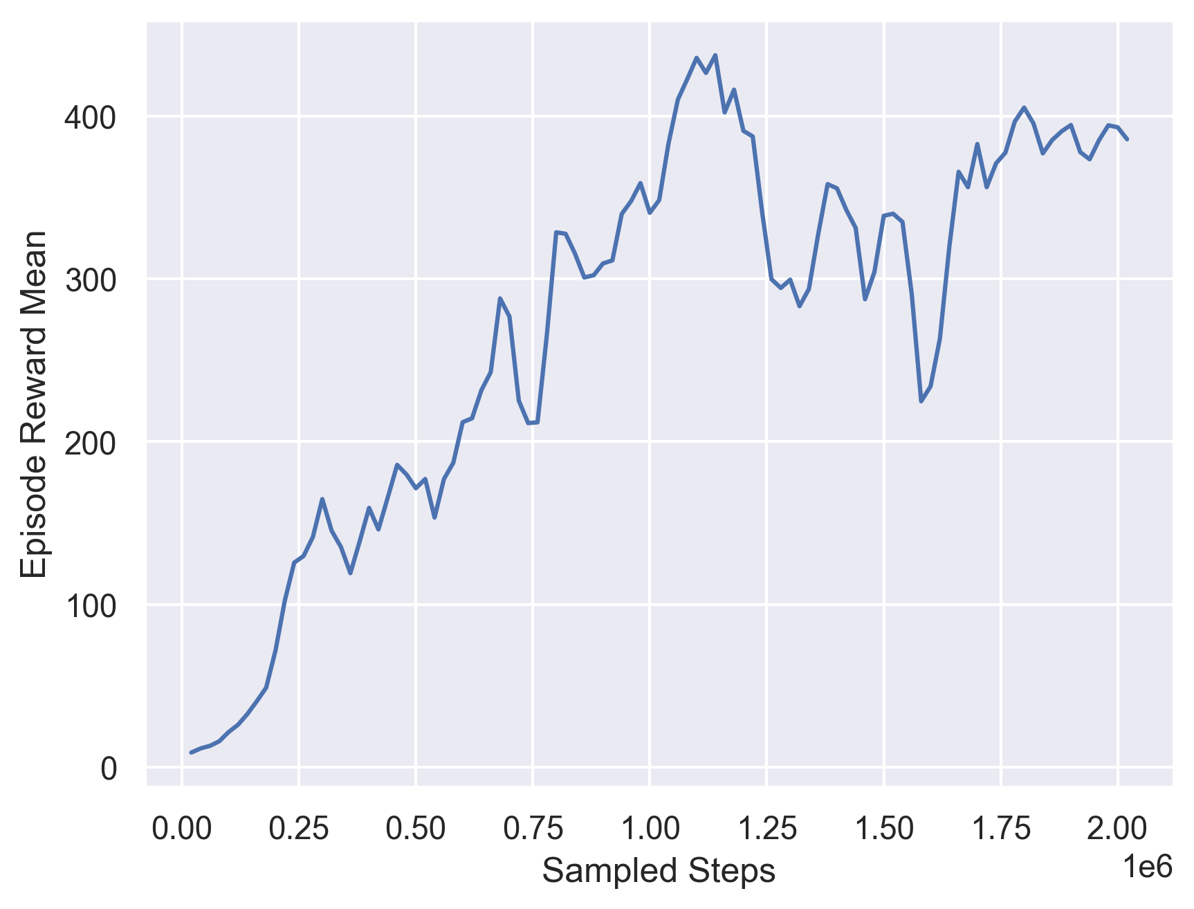
Fig 11. Training Curve for a PPO on Circular and Roundabouts Road Environments.
We could find that the training awards is very high since the training senario is simplified, but they cannot generalize to more complicated evaluation environments and the corresponding evaluation rewards are low.
We then train the selection model based on these three baseline models. The training curve for this model is showed below and the evaluation episodic reward is 146.103.
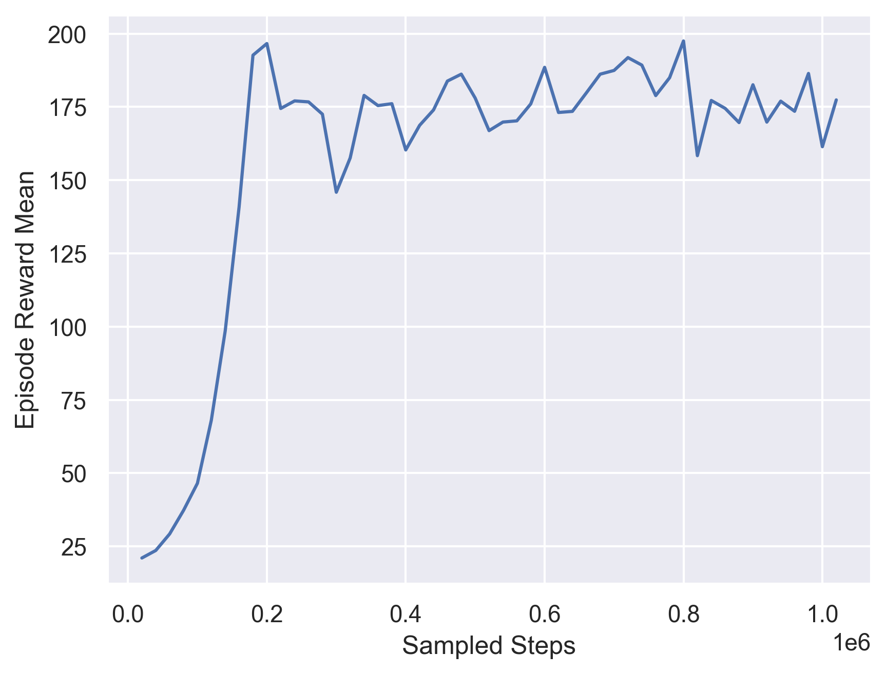
Fig 12. Training Curve for a PPO Seletion Model.
We find that the overfitting problem is much better in this case. For the performance, we find that the performance is between the best cases and worst cases. This might due to our limited evaluation environments.
We also plot visualize the model on one of our evaluation environments. We also show the weights assigned to different baseline models and the dominante model.
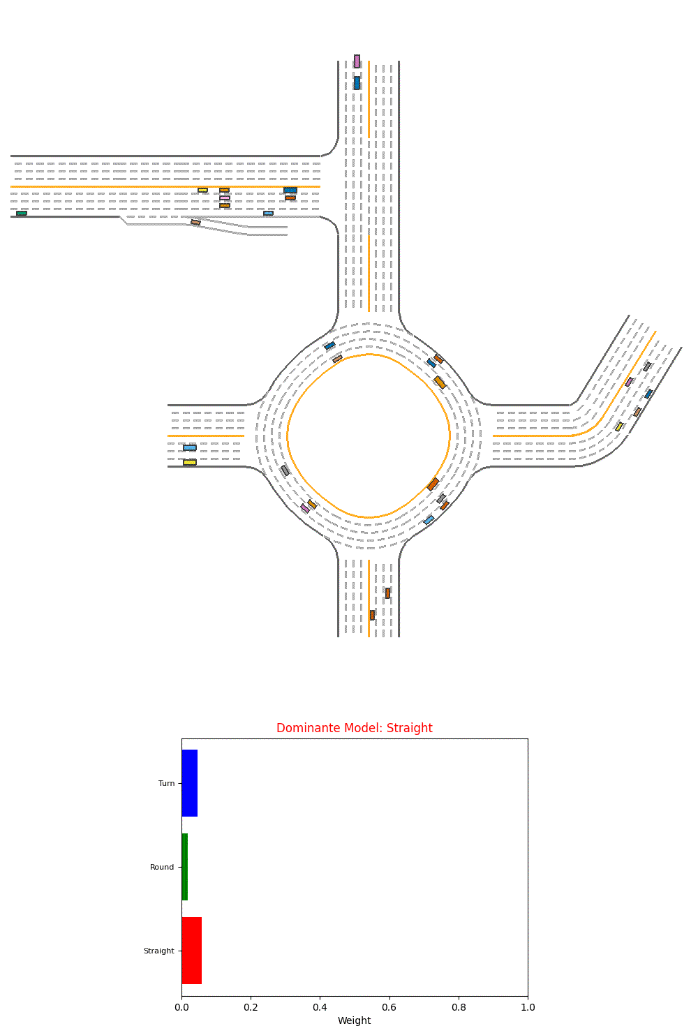
Fig 13. Visualization of Performance of a Single PPO agent.
However, we could see from the visualization that it’s more generating random weights and could not select the best model so far.
4.3.3 Ensemble Different PPO Models Trained on Different Traffic Situations
In addition to the ensemble of multiple models, we also experimented with ensemble of models trained with specialization on traffic situations.
4.3.3.1 Environments
In this experiments, we uses environments configured from MetaDrive-Tut-100Env-v0 above.
To create specialized environments, we create environments with roads with 2, 3, 4 lanes, and the traffic density between 0.005, 0.01, 0.02 cars per 10 meters.
This gives us a total of 9 specialized environments, named with format MetaDrive-XHard-{}Lane-{}Traffic-v0.
The general environment, created from by sampling each of the 9 specialized environments randomly, is named MetaDrive-XHard-v0.
4.3.3.2 Specialized models
We trained a specialized model for each of the specialized environment above. They are PPO models, trained with 4,000,000 time step with the same hyperparameters as the experiment before.
4.3.3.3 Generalized models
Similar to above, we have the following attempted generalized model:
- The PPO model, a model trained with the same architecture as the specialized model, to use as a control.
- The average Generalized ensemble, a model created by using 9 PPO models on the generalized environment.
- The PPO-weighted Generalized ensemble model, a model that uses PPO to select weight for the weighted average from 9 PPO generalized models.
- The average Specialized ensemble, a model created by using equal-weighted average from specialized models.
- The PPO-weighted Specialized ensemble model, a model that uses PPO to select weight for the weighted average from specialized models.
We have considered increasing the size of the single PPO model, but 1) we do not know what exact architecture would make a fair comparison, and 2) we are constrained by our computation resources. Also, we tried to give the single PPO model an extra 1,000,000 steps of training, to be consistent with the training used by the weight-selection PPO, but the training did not give better result.
We did not perform hyper-parameter tuning; all the parameters are the same as the model used in assignment 3. However, we might select best model based the training rewards.
We have also added a softmax layer after the weight-selection model to ensure each output weight is positive and sum as 1, yet it does not produce better results.
4.3.3.4 Results for Specialized models
The results are shown in the following table:
| MetaDrive-XHard Models | Training Reward | Training Success Rate | Evaluation Reward |
|---|---|---|---|
| 2Lane-50Traffic-v0 | 327.821 | 0.9 | 319.938 |
| 2Lane-100Traffic-v0 | 297.117 | 0.71 | 238.255 |
| 2Lane-200Traffic-v0 | 265.671 | 0.57 | 252.963 |
| 3Lane-50Traffic-v0 | 305.523 | 0.69 | 289.463 |
| 3Lane-100Traffic-v0 | 303.550 | 0.74 | 312.993 |
| 3Lane-200Traffic-v0 | 262.572 | 0.57 | 234.864 |
| 4Lane-50Traffic-v0 | 313.710 | 0.61 | 306.772 |
| 4Lane-100Traffic-v0 | 266.616 | 0.33 | 239.655 |
| 4Lane-200Traffic-v0 | 255.887 | 0.4 | 217.981 |
Table 4. Experiment Result for PPO Model Trained in Each Specialized Environment.
4.3.3.5 Results for Generalized models
The results are shown in the following table.
The single PPO are reported as a distribution from the 9 models, in format of (min, mean, max)
| Models | Training Reward | Training Success Rate | Evaluation Reward |
|---|---|---|---|
| Single PPO | (171.324, 224.220, 281.097) | (0.11, 0.33, 0.53) | (166.909, 221.985, 259.975) |
| Average Specialized Ensemble | N/A | N/A | 174.157 |
| PPO Specialized Ensemble | 284.916 | 0.58 | 273.120 |
| Average Generalized Ensemble | N/A | N/A | 228.523 |
| PPO Generalized Ensemble | 279.211 | 0.58 | 275.704 |
Table 5. Experiment Result for models trained in the generalized environment.
And the correponding training Curves for Single PPO model:
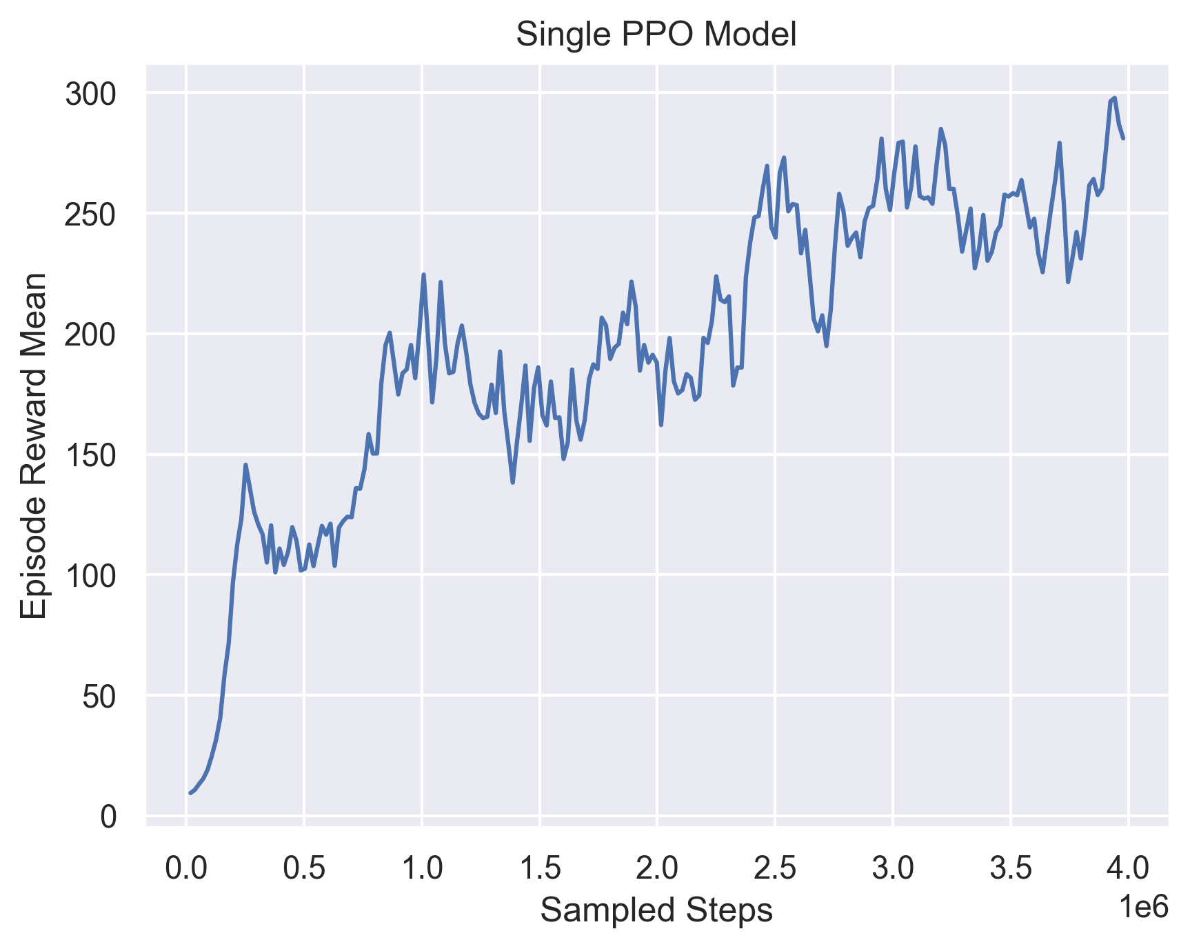
Fig 14. Training Curve for a single PPO model.
And the correponding training Curves for Ensemble PPO model:
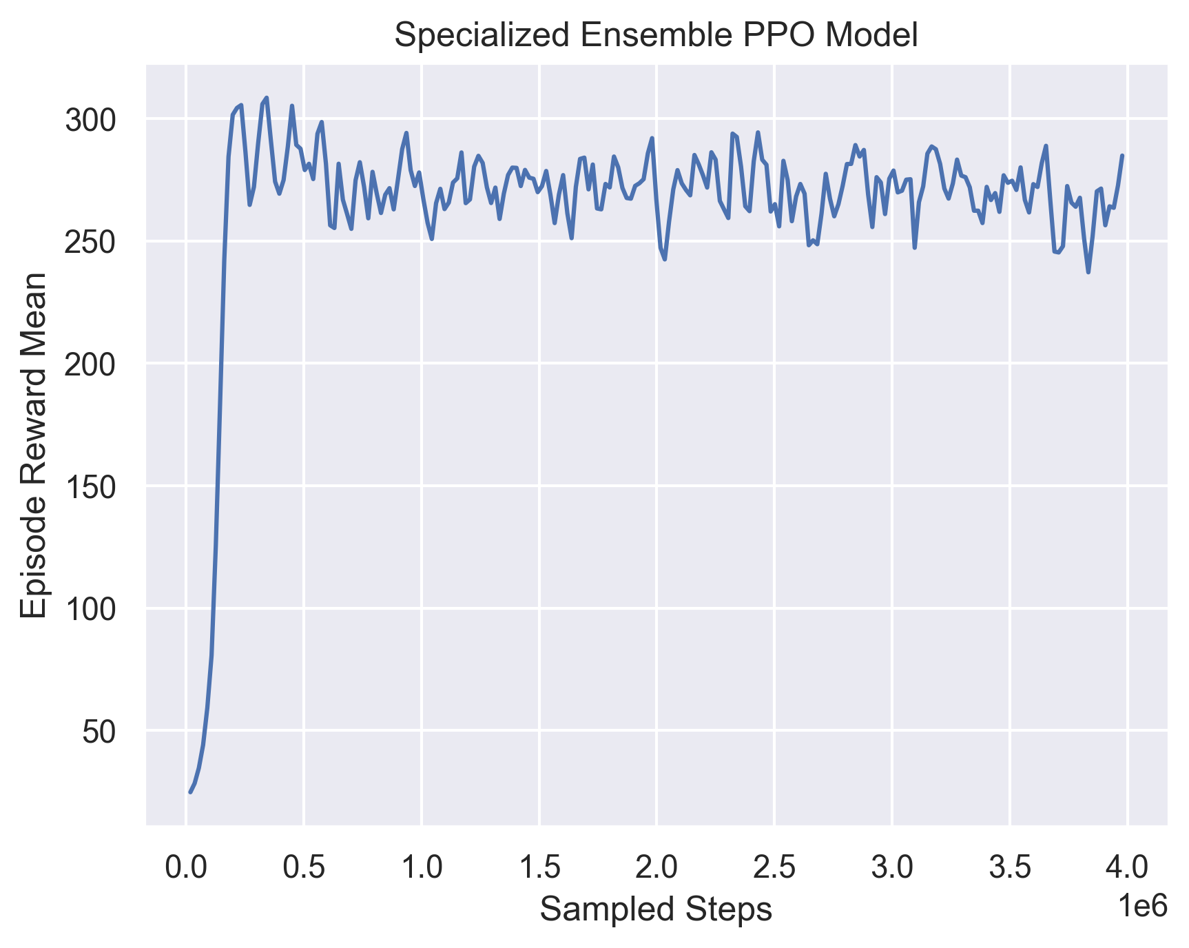
Fig 15. Training Curve for training weight-selection model with specialized submodels.
And the correponding training Curves for Generalized Ensemble PPO model:
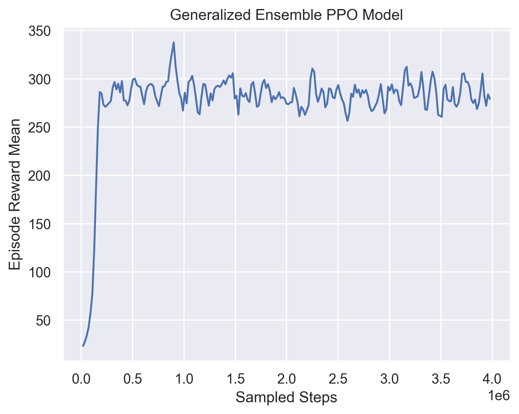
Fig 16. Training Curve for training weight-selection model with generalized submodels.
We can see that the average ensemble models does not perform better than the single PPO in general. The ensemble models performs much better than the other models in evaluation, and in between them, the specialized ensemble performs slightly better, probably because it is able to accommodate more edge cases.
Another thing we can notice is that the ensemble models have a smaller gap between training and evaluation rewards, compared to the single models. For the best model in Single PPO, it can achieve 281.087 in training, but only at most 258.975 in evaluation, while the ensemble models have the a gap of less than 5.
4.3.3.6 Visualization
We continue to use the visualization from the above experiment, but modified to use 4 Lanes and 0.2 cars per 10 meters. This is the cases where the specialized model has the lowest score.
For the single agent(Using the highest evaluation reward model), the model achieves 171.969 reward.

Fig 17. Visualization of Performance of a Single PPO agent.
For the average generalized model, the model achieves 482.650 reward.

Fig 18. Visualization of Performance of Averaging Ensemble over generalized models.
For the PPO generalized ensemble, the model achieves 518.062 reward.

Fig 19. Visualization of Performance of PPO weight-selction Ensemble over generalized models.
For the average specialized model, the model achieves 429.753 reward.
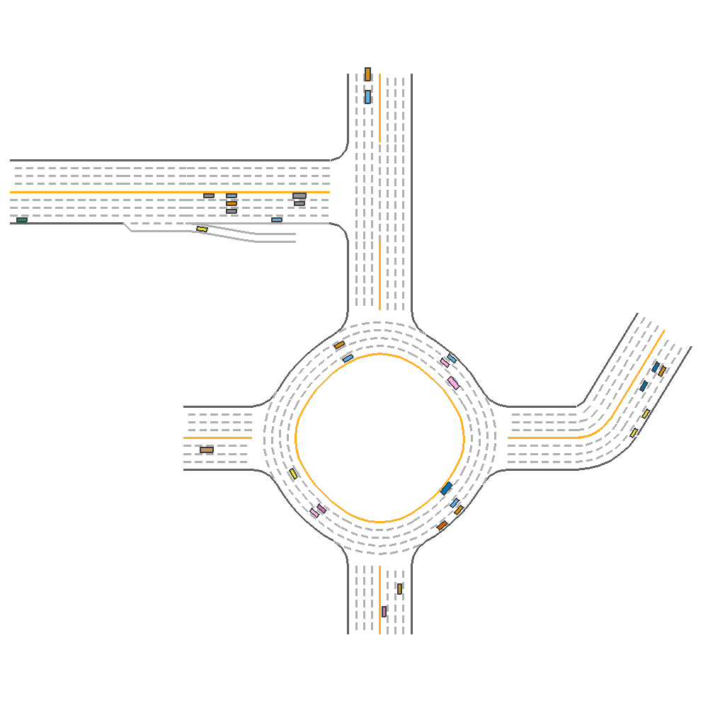
Fig 20. Visualization of Performance of Averaging Ensemble over specialized models.
For the PPO specialized ensemble, the model achieves 526.172 reward.
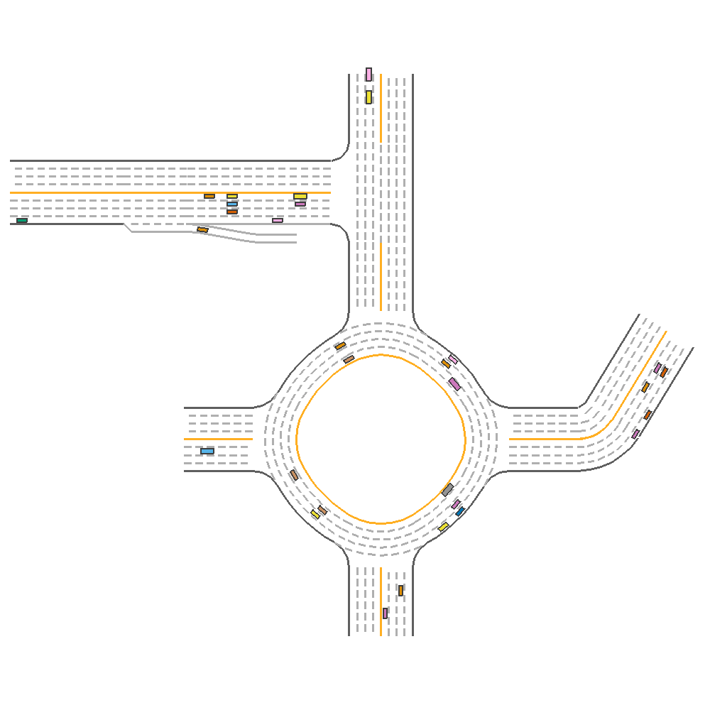
Fig 21. Visualization of Performance of PPO weight-selction Ensemble over specialized models.
In this, we can see that both ensemble model is able to arrive at the destination correctly. The average models almost reached the destinations, and the single agent have failed to move through.
4.3.3.7 Trained Weight analysis
We can also visualize the weight selection by the weight-selection PPO model. Because the original weight output from the model is too jittery, we use a exponential moving average to smooth the weights. The alpha used in moving average is 1/8.
For the scenario in the visualization case, we outputted the weight.
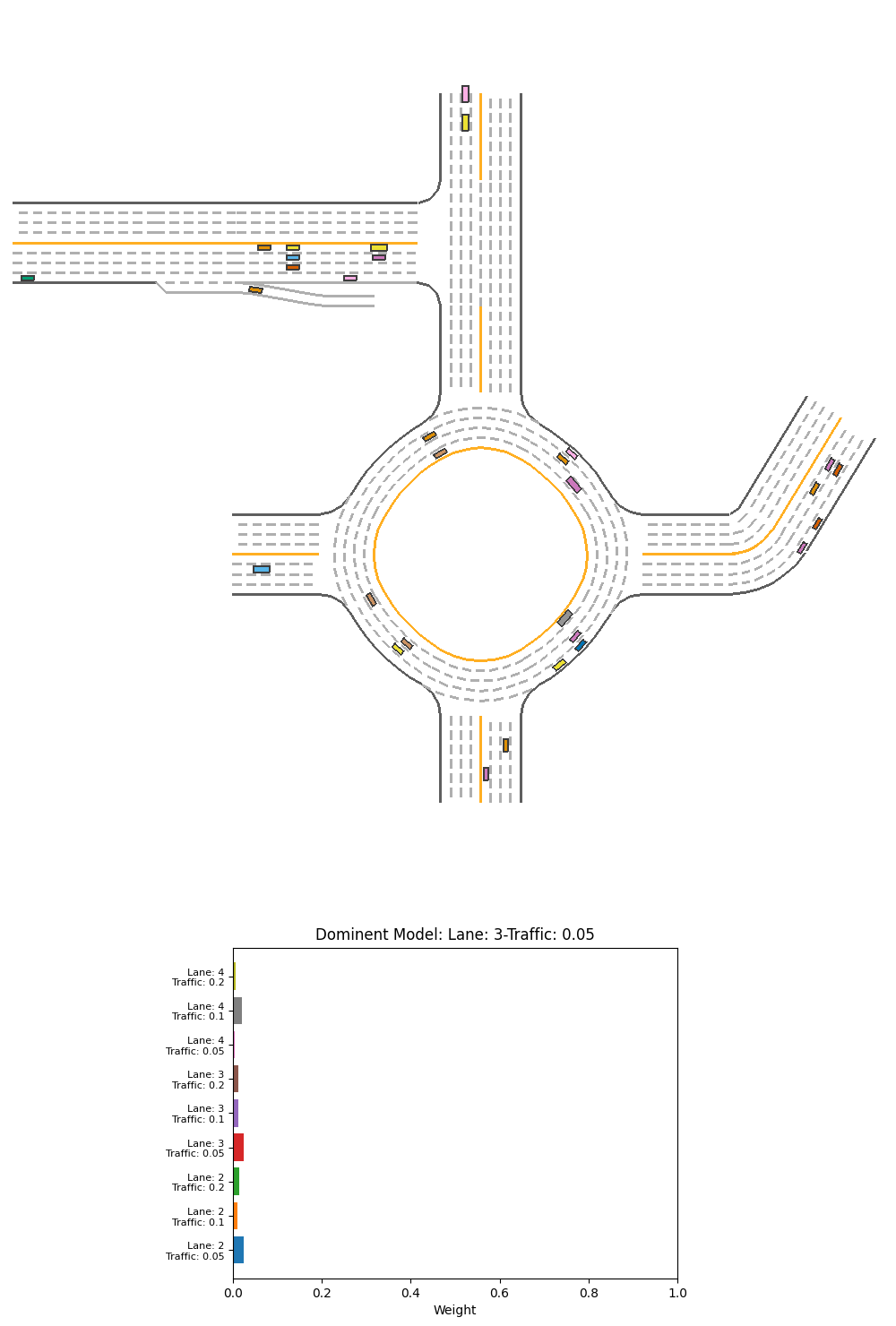
Fig 22. Performance and corresponding output weight of PPO weight-selction Ensemble over specialized models on 4-lane heavy-traffic scenario.
From this visualization, we do not see the weight pattern for recognizing this scenario as 4-lanes, or as a scenario of heavy traffic. We only see that the 3-lane mid-traffic model is used the most overall, probably as the default when there is no obstacles. However, there are some patterns that are not evident at certain key areas of the driving:
- At the T-section turning, the right turn is started by the high weight of 2-lane models, pulling the car to the side line.
- When the car is sourrounded by traffic after the T-section or after the roundabout, we see the 3-lane medium or heavy-traffic models are given more weight.
We have also visualize the 2-lane scenario, which are driven poorly by the car.
For the scenario that reduces number of lane to 2, we see the car failed and have only 96.603 reward.
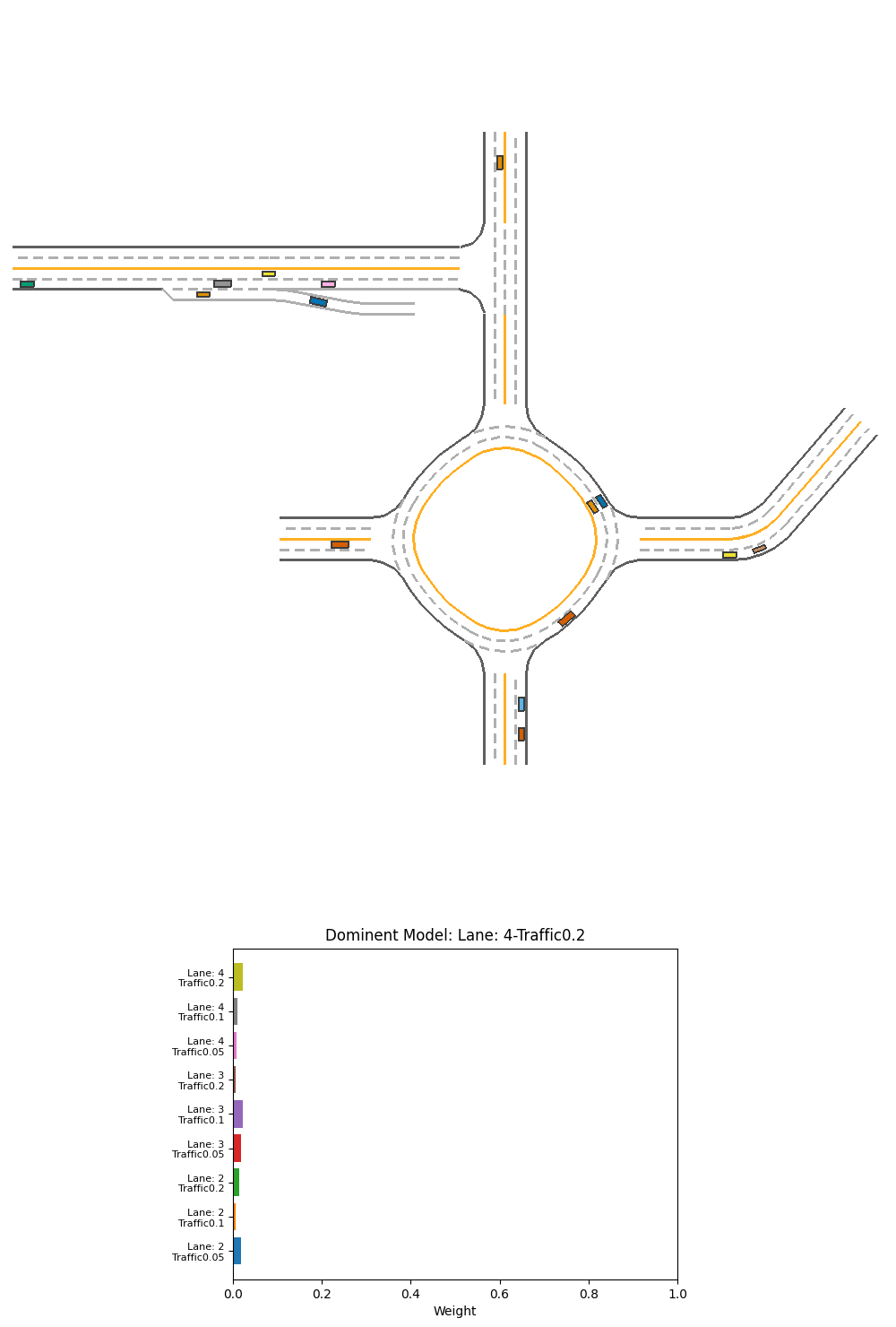
Fig 23. Performance and corresponding output weight of PPO weight-selction Ensemble over specialized models on 2-lane heavy-traffic scenario.
For the scenario with 2 lanes and 0.05 traffic, we see the car failed and have only 95.184 reward, and the failure trajectory is about the same as the 2-lane heavy traffic scenario.
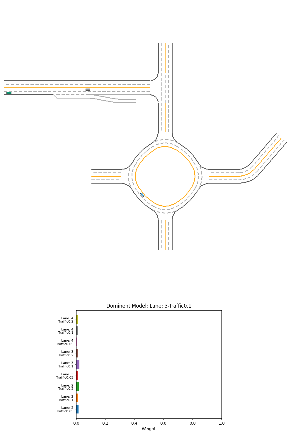
Fig 24. Performance and corresponding output weight of PPO weight-selction Ensemble over specialized models on 2-lane light-traffic scenario.
For the above 2 scenarios, we can see the cars have hit the mid-line. Before the crash, we can see that the 3 or 4-lane models have a equal or even slightly higher weight than 2-lane models. It is probably the 3 or 4-lane model tries to avoid the exit and go back to the middle of the imaginary 3 or 4-lane road, which crashes the vehicle into the midline. The model did not seems to learn that the 2-lane model’s input is better in this case.
4.3.3.8 Analysis
We do see that our ensemble model is able to perform better than the single agent model. However, this better performance is mostly because of the robustness created by the use of differently trained model. We do not see an interpretable pattern of weight-selection model recognizing the lane-number and traffic amount; instead, it starts to optimize toward the easier cases (high lane number), where policy changes in those can increase reward faster than in those harder cases. We also see some weight patterns for specifically avoiding certain obstacles.
5 Conclusion and Future Works
In summary, in this project, we tried different ways to ensemble several different reinforcement learning model. Most ensemble method achieve similar or slightly better result than the best baseline models. But in all ensemble is not very effective in increasing the performance in autonomous driving tasks. But we still see good sign for the potentials in improving. Due to our device constraints, we are not able to train all the models until convergence for many models. Therefore, there may be room for improvements for our PPO models. We also do not have enought time for model tuning. Also our testing environments are limited and thus may result in randomness of the result.
Based on the ensemble model on different traffic situation, in the future, we may consider
- Increase the importance of difficult scenarios by multiplying the reward.
- Allow the scenario to continue after the car crashes, but give some penalty. This allows the model to see the rewards after the crash, and not limited by the difficult problem in the beginning. It is also implemented in the Safe driving environment in Metadrive.
- Instead of use pretrained models, we can train the base model and the selection model together.
6 Video Demo
Please kindly check the following link:
Video Click Here,
Demo PPT Click Here
7 References
- John Schulman, Filip Wolski, Prafulla Dhariwal, Alec Radford, & Oleg Klimov (2017). Proximal Policy Optimization Algorithms. CoRR, abs/1707.06347.
- Fujimoto, S., Hoof, H., & Meger, D.. (2018). Addressing Function Approximation Error in Actor-Critic Methods.
- Ho, J., & Ermon, S.. (2016). Generative Adversarial Imitation Learning.
- Haarnoja, T., Zhou, A., Abbeel, P., & Levine, S.. (2018). Soft Actor-Critic: Off-Policy Maximum Entropy Deep Reinforcement Learning with a Stochastic Actor.
- Dietterich, T.G. (2000). Ensemble Methods in Machine Learning. In: Multiple Classifier Systems. MCS 2000. Lecture Notes in Computer Science, vol 1857. Springer, Berlin, Heidelberg. https://doi.org/10.1007/3-540-45014-9_1
- Dosovitskiy, A., Ros, G., Codevilla F., Lopez A. & Koltun V.. (2017). CARLA}: An Open Urban Driving Simulator. In Proceedings of the 1st Annual Conference on Robot Learning, page 1-16.
- Li, Q. and Peng, Z. and Xue, Z. and Zhang, Q. & Zhou, B.. MetaDrive: Composing Diverse Driving Scenarios for Generalizable Reinforcement Learning. In arXiv preprint. arXiv:2109.12674.
- Vinitsky, E., Lichtlé, N., Yang, X., Amos, B. & Foerster, J.. Nocturne: a scalable driving benchmark for bringing multi-agent learning one step closer to the real world. In arXiv preprint. arXiv:2206.09889.
- Zhou, M., Luo, J., Villella, J., Yang Y. & Rusu, D., et al. (2020). SMARTS: Scalable Multi-Agent Reinforcement Learning Training School for Autonomous Driving. In Proceedings of the 4th Conference on Robot Learning (CoRL).
- Shah, S., Dey, D., Lovett, C. & Kapoor, A. (2017). AirSim: High-Fidelity Visual and Physical Simulation for Autonomous Vehicles. In Field and Service Robotics. arXiv:1705.05065.
- The Ray Team. Algorithms - Ray 2.1.0. Accessed Dec 9, 2022. https://docs.ray.io/en/latest/rllib/rllib-algorithms.html#model-based-meta-policy-optimization-mb-mpo.
- Sagi, O. and Rokach, L.. (2018). Ensemble learning: A survey. In WIREs Data Mining and Knowledge Discovery.
- Wiering, M. and van Hasselt, H.. Ensemble Algorithms in Reinforcement Learning. In IEEE Transactions on Systems, Man, and Cybernetics, Part B (Cybernetics), vol. 38, no. 4, pp. 930-936, Aug. 2008, doi: 10.1109/TSMCB.2008.920231.
- Kimin Lee, Michael Laskin, Aravind Srinivas, Pieter Abbeel. (2021). SUNRISE: A Simple Unified Framework for Ensemble Learning in Deep Reinforcement Learning In Proceedings of the 38th International Conference on Machine Learning, PMLR 139:6131-6141.