Planning with Learned Actionable Object-centric World Model
To achieve better planning in zero-shot generalization RL tasks, we propose to learn imagined actions over perceived objects in the learned world model. We first reproduced the work Veerapaneni et al’s OP3 method ([5]), which learns a general object-centric world model. Then we implemented our proposed model design to enable the imagined action. We trained it with the block stacking task that the OP3 work has been evaluating on to make sure our method still performs correctly. Our method can still work correctly to learn meaningful representations that can be used to reconstruct the original image, and the forward dynamics are correct. But the imagined action doesn’t work well yet, which we suspect due to both the poorly fitted prior and the limitation of the dataset. We have been trying to create a billiard ball environment, but due to unexpected bugs and time constraints, we have not finished. When it’s finished we can check our imagined action method a lot more intuitively.
Project Proposal
Model-based RL can improve data efficiency and reduce the amount of data needed when switching to a new environment, but for the zero-shot scenario, it doesn’t necessarily generalize to a new world different without extra techniques ([2], [3]). Recently, some model-based works take the object-centric approach to learning world models in multi-object settings and achieve much better zero-shot generalization performance since such world models can much more easily adapt to different numbers of objects ([1], [4], [5]). However, the objects in the current object-centric world model are treated implicitly and can’t be utilized explicitly for planning. People still have to treat the entire object-centric world model as one black box, just like other kinds of world models during planning.
To achieve better planning in zero-shot generalization tasks, we propose to learn imagined actions over perceived objects in the learned world model. The imagined action is an interface to imagine how the object could be changed regardless of how it’s achieved (the agent would change it, and the other objects can also affect it). Then, we can imagine first what ‘action’ should the goal object take to achieve the goal state, and then imagine what other object should ‘act’ to provide the goal object’s desired action, and iteratively all the way back to the agent’s own action space. In this way, especially in the multi-object control task, the exponentially complex planning task is decomposed into sub-problems that each is easy to plan.
We have implemented our method based on Rishi’s OP3 method ([5]), which learns a general object-centric world model structure. We will create a billiard ball environment to test and improve the algorithm in the future.
Note: we intend this project to be a fully academic project and publish later. We’d appreciate our fellow classmates to keep the content confidential.
Algorithm
Reconstruction of OP3 Algorithm
To incorporate our ideas to the existing OP3 algorithm, we first reconstructed it to obtain a better understanding from the detailed implementation. The foundation of this algorithm is the symmetric entity abstraction assumption. That is, the algorithm can learn an entity-centric model, from a single object along with its interactions, which can then be applied to every object in the scene ([5]). The main structure is the iterative amortized inference with three modules embedded: recognition, dynamics, and observation.
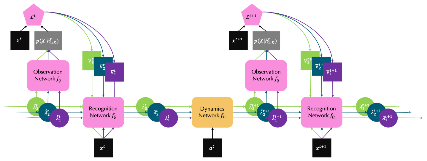
Figure 1. Main Structure of OP3 Algorithm
Flow of the main structure
Given an image of the initial state of a dynamic process, \(x^0\), the recognition network is able to learn a latent encoding for each object in the current scene, \(\lambda_{1:K}^0\). Then the dynamics network is responsible for constructing a world model, i.e., predicting the future latent state of each object after some action \(a^0\) applied, \(\hat{\lambda}_{1:K}^{1}\).
Next, the observation network is going to reconstruct the image for the next time step, \(x^1\), by applying the same object-centric function to each of the predicted encodings, \(\hat{\lambda}_{1:K}^{1}\). Specifically, it reconstructs every object individually and associates with a segmentation mask deciding its depict in case of occlusion.
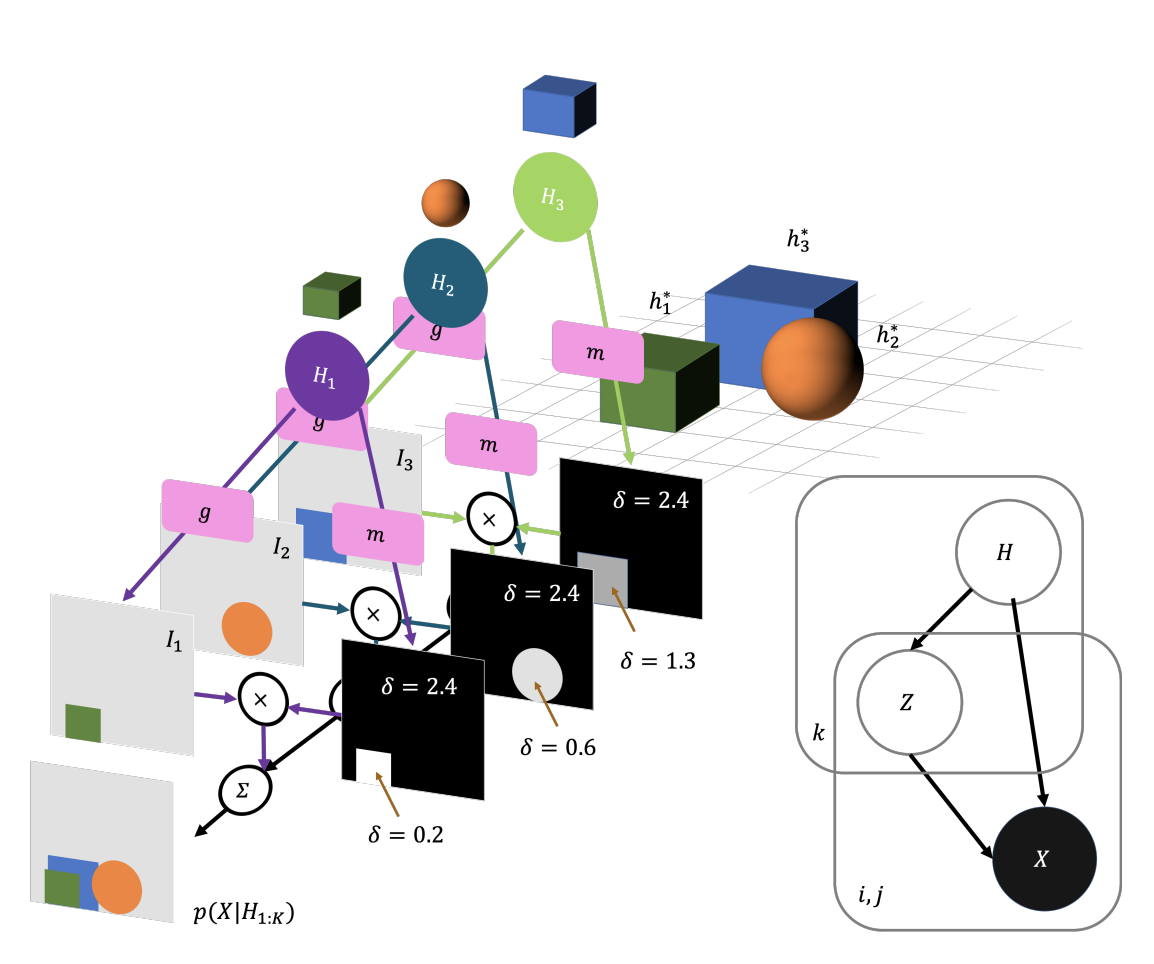
Figure 2. Observation Network of OP3 Algorithm
Finally, the recognition network takes the predicted encodings from the dynamics network, \(\hat{\lambda}_{1:K}^{1}\), the reconstruction errors from the observation network, \(\nabla_{1:K}^1\), and the raw image, \(x^1\), to further refine the encodings, \(\lambda_{1:K}^{1}\). It is worthy noticing that this refinement procedure will break the symmetry among objects due to the noise introduced by the predicted encodings. The whole process continues until it reaches the last frame in the sequence.
To summarize, OP3 algorithm is composed of two main steps: the dynamics step and the refinement step. As shown in Figure 1, the dynamics step includes only the dynamics network, while the refinement step includes both the observation and the recognition networks. Next we will dig into more implementation details for each step.
Dynamics step
The dynamic module learns a world model to predict each object latent encoding for the next state locally (without using any pixel information). It starts with modeling how the given action intervenes each object, and then considers how objects interact with each other pairwisely.
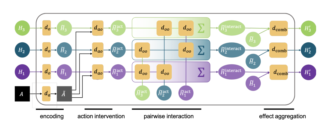
Figure 3. Dynamics Network of OP3 Algorithm
The specific procedure is as follows:
- Objects and action encoding:
\begin{aligned} \tilde{H_k} &= d_o(H_k),\\ \tilde{A} &= d_a(A) \end{aligned} - Action intervention:
Measures how and to what degree an action \(A\) affects the object \(H_k\).
\begin{align} \tilde{H_k}^{act} &= d_{ao}(\tilde{H_k}, \tilde{A})\\ &:= d_{act-eff}(\tilde{H_k}, \tilde{A}) \cdot d_{act-att}(\tilde{H_k}, \tilde{A}) \end{align} - Pairwise interaction:
Measures how and to what degree other objects affect the object \(H_k\).
\begin{aligned} \tilde{H_k}^{interact} &= \sum_{i\neq k}^Kd_{oo}(\tilde{H_i}^{act}, \tilde{H_k}^{act})\\ &:= \sum_{i\neq k}^K[d_{obj-eff}(\tilde{H_i}^{act}, \tilde{H_k}^{act}) \cdot d_{obj-att}(\tilde{H_i}^{act}, \tilde{H_k}^{act})] \end{aligned} - Pairwise interaction VAE (newly added):
Note: The original OP3 algorithm learns a specific pairwise interaction, so it does not contain this step.
Instead of learning the specific pairwise interaction, the model learns a probabilistic version of it, i.e., the parameters of its distribution, \begin{aligned} f(\tilde{H_k}^{interact}). \end{aligned} Then we sample from this distribution \begin{aligned} \tilde{H_k}^{interact(sampled)}\sim f(\tilde{H_k}^{interact}). \end{aligned} - Effect aggregation:
\begin{aligned} H_k’=d_{comb}(\tilde{H_k}^{act}, \tilde{H_k}^{interact(sampled)}) \end{aligned} - Posterior sampling of the next state:
\begin{aligned} H_k’^{(sampled)}\sim f(H_k’) \end{aligned}
Refinement step
The refinement step in OP3, i.e., the observation network and the recognition network, is based on the IODINE algorithm for learning image segmentation of occluded objects with disentangled representations as shown below ([7]).
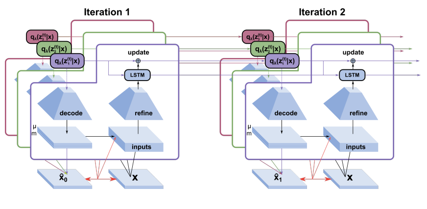
Figure 4. IODINE Algorithm
The formula for updating the next iteration in IODINE is: \begin{aligned} z_k^t &\sim q_H(z_k^t | x)\\ H_k^{t+1} &\leftarrow H_k^t + f_\theta (z_k^t, x, a_k) \end{aligned} where \(z_k^t\) is the sampled encoding of object \(k\) from the distribution \(H\) given \(x\) at \(t\) step, and the \(H_k\) updates itself through an neural network \(\theta\) that takes in its previous step’s sample \(z_k\), the image \(x\), and other inputs \(a_k\) which includes gradients, masks, loss etc.
The loss function to optimize for IODINE is to minize the evident lower bound (ELBO) like the standard VAEs. \begin{aligned} L_t = D_{KL}(q_H(z^t|x) || p(z)) - log p(x|z^t) \end{aligned} where \(p(z)\) is a normal distribution in this setting.
Object-centric planning
After training, OP3 method can extrapolate to novel scenes with no extra scene-specific training needed. In other words, it learns to plan actions from only the goal-state image. In particular, it tries a bunch of random actions and uses the learned OP3 model to simulate the final results respectively. Then it picks the best several actions and sample another batch of random actions using the cross-entropy method (CEM). Theoretically, the newly sampled actions, although random, are improving iteratively. The way it defines “better” among actions is by a smaller error between the simulated object encoding in the final state and the one inferred from the goal-state image directly. During planning, the whole OP3 model learned from training remains a blackbox, with the initial-state image and an random action as the inputs and the predicted final-state object encodings as the outputs; that is, it does not uitilize any object representation learned explicitly.
Our Results
##### For comparison purpose, we keep with two of the environments (tasks) in MuJoCo from the original OP3 paper, block stacking and pick place. In the block stacking task, a block is raised in the air and the model is going to predict the scene after the block dropped, so the model needs to understand gravity and collisions ([5]). The pick place task is a modified version of multi-step block stacking, which extends the action space to include a picking and dropping location, so the agent may have to manipulate more than one block to reach the goal state ([5]).
The following images compare the training results in each task using the original model in the paper with the ones using our modified VAE version of the model. And it demonstrates that the model maintains the quality of performance even if we use variational encoding and sampling for the pairwise interaction. Particullarly, the reconstruction and prediction of our modified model are quite accurate compared to the ground truth for a large range of tasks.
Block stacking
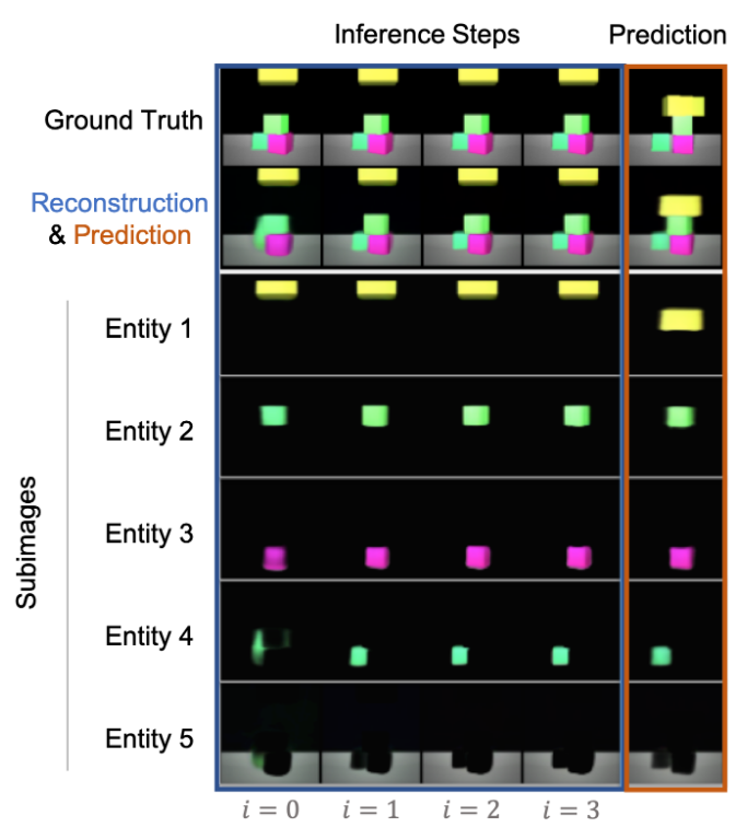
Figure 5. Training Result of Block Stacking in the Original Paper

Figure 6. Training Result of Block Stacking Using Modified VAE Model
Pick place
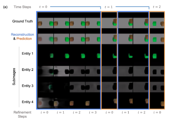
Figure 7. Training Result of Pick Place in the Original Paper
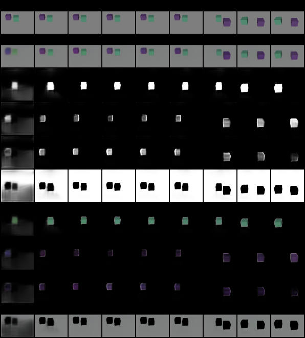
Figure 8. Training Result of Pick Place Using Modified VAE Model
Note: in the example shown in Figure 8, the first 6 frames are one set of refinement steps, then the 7th frame is one time step forward (1 dynamics step, no refinement), and finally the last 2 frames are one more time step forward along with 1 refinement step.
Model Improvements and Corresponding Results
1. To be able to imagine (plan) the actions or interventions over any specific object, we need to first have a method for generation.
Variational encodings with forced normal distribution prior seems to be a good way to achieve this purpose. Suppose the action encodings are trained well and close enough to normal distribution, we would have a known prior that we can sample from to generate various actions.
To test our hypothesis, we started with investigating the variational encoding and its representation power. In particular, we made an experimental move by adding variational encoding to the object’s pairwise interaction in the dynamics network. The improvement and results are shown in the above reconstruction session.
2. Besides, to prevent bad extrapolation, we need a unified action interface that can be controlled easily for diverse actions.
Since we can guarantee to reproduce only the type of effects (changes in images) of actions experienced during the training process, we want to feed in as diverse actions as possible and make sure they cover all potential kinds of changes. However, the original dynamics network in OP3 models the effect of an action on all the objects in the scene as a chain. In specific, it combines action intervention first and then pairwise interaction. In this case, there is no guanrantee that different actions will lead to difference effects, because the interaction part is hard to control.
Instead, our model learns a unified action interface, which is more physically realistic (in the sense that both action intervention and pairwise interaction are just forces after all) and also more elegant. The following are the improvements based on the modified version of OP3 dynamics network shown in the previous reconstruction session.
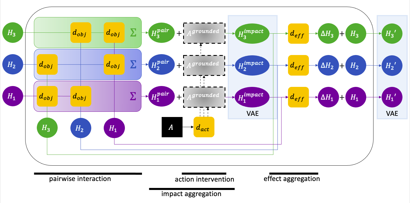
Figure 9. Improved Dynamics Network
Note: please compare to Figure 3 to see the improvements more clearly.
- We skipped the entities encoding that accounts for the inertia in the original algorithm because we want it to be implicitly learned in one same network that accounts for the actions effect. That means, when the action is absent, that network should output the effect from the inertia.
- Action intervention:
In our design, the action come from an agent that’s either also in the scene or can only affect one object at a time. So we want to ground the actions on to the object it affect (the object could be agent itself). So we use an attention to select the object to affect on. We also encode the action to be a vector encoding like the old algorithm, but we don’t hurry to apply the action to objects and get an updated object encoding for now. \begin{aligned} A^{grounded} = d_{act-enc}(A) \cdot d_{act-att}(H_{1:K}, A)
\end{aligned} - Pairwise interaction:
We still want to measure how and to what degree other entities affect the entity (H_k). This interaction is not from agents actions of course. \begin{aligned} H_k^{pair} = \sum_{i\neq k}^K[d_{obj-imp}(H_i, H_k) \cdot d_{obj-att}(H_i, H_k)] \end{aligned} - Impact aggregation:
This is also where we are different. We treat impact from action and from objects’ interaction to be intrinsically same type (intuitively, they are all just force). For terminology wise, we use “impact” to denote this general force from both action and interaction. In this step, we aggregate both kinds of impacts toward a specific entity (H_k) by simply adding them up: \begin{aligned} H_k^{impact} = A^{grounded} + H_k^{pair} \end{aligned} - Total impact VAE:
In this step we turn the aggregated impact into a variational encoding. This is how we manage to have one unified “action” interface toward any object. No matter where the original impact come from (from agents’ actions or objects interactions), the aggregated impact at any time step must follow a prior distribution. Thus we create an interface to intervene the object agnostic to the impact source, and thus we can imagine intervening the objects later. \begin{aligned} H_k^{impact(sampled)}\sim f(H_k^{impact}). \end{aligned} - Update the objects by applying the impact:
At this step we apply the aggregated impacts toward the object to update its state. We use a network with the object’s previous state (H_k) and the total impact sampled from the learned distribution (H_k^{impact(sampled)}) as the inputs and compute the state change. And then we add the state change to it to get the object’s next state. \begin{aligned} \Delta H_k&=d_{effect}(H_k^{impact(sampled)}, H_k)\\ H_k’&=H_k+\Delta H_k \end{aligned} - Posterior sampling of the next state: This part remains the same. \begin{aligned} H_k’^{(sampled)}\sim f(H_k’) \end{aligned}
3. Some characteristics of an object may not change while an action applied, so they can be spared from the dynamics network.
For example, in the block stacking environment, the shape and color of each block should always remain the same. Thus, they are only useful for reconstruction purpose, but should be steady for prediction. Figure 10 depicts our improvement of the main iterative amortized inference structure. Here \(AP_{1:K}\) represent the appearance of each object. Since no matter how many time steps passed, the appearance of an object should remain untouched, there is no need of a superscript for time. As shown in the graph, the appearances do not pass through the dynamics network, but they do get refined through observation and recognition networks.
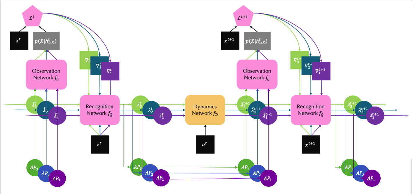
Figure 10. Improved Main Structure
Note: please compare to Figure 1 to see the improvements more clearly.
Results
The following images are the reconstruction and prediction of a training scene and a validation scene in the block stacking and pick place tasks respectively. All 4 of them produce relatively accurate final-state images compared to the ground truth. This illustrates that our improved model carries on the performance of the original OP3 model.
Block stacking

Figure 11. Training Result of Block Stacking Using Improved Model

Figure 12. Validation Result of Block Stacking Using Improved Model
Pick place
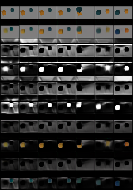
Figure 13. Training Result of Pick Place Using Improved Model
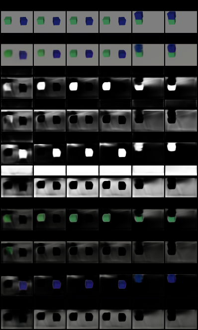
Figure 14. Validation Result of Pick Place Using Improved Model
Challenging Scenes
For complex scenes where there’re many objects and skewer positions, however, the performance have not reached a perfect state yet. But we estimate with more training and data the problems would be solved as wee can see from the images that they seem to be getting there.

Figure 15. Training Result of Block Stacking Using Improved Model In Complex Scene
Apply Random Imagined Actions to Objects
We want to test applying random impacts/actions to objects and seee their reconstruction results. Unfortunetaly it hasn’t demonstrate a good behavior yet. As we can see from the image the objects become a lot more blurer when we apply random action/impacts onto the objects. It might because the learned VAE action interface does not perfectly fit the prior distribution. The dataset itself might also be a problem since the interactions among objects are not diverse (generally only the dropped block move and always move down), so it might be hard to learn various possible actions.

Figure 16. Applying Random Impact/Imagined-Actions to Blocks Using Improved Model
Billiard Ball Environment
In this section, we introduce a new environment – billiard ball (BiB) game environment , which is implemented based on two similar existing environments: Bouncing Ball (BB) [9] and Pool Game (PG) [10]. We have not fully made it work and compatible to our RL training workflow but it’s almost there.
We stipulate the billiard ball game environment to:
- There is only one white ball serving as a cue ball that will be applied with the initial velocity generated by the model or randomness after each hit action.
- There are one to infinite number(s) of the solid color ball(s) serving as the objective balls(s) that will be placed randomly on the billiard ball table at the beginning of each game.
- There are at most six pocket(s) on the billiard ball table located at the top, middle, and bottom.
We define the billiard ball game rules to:
- Our goal is to hit all solid color ball(s) into the pocket(s) with the direct help of the white ball or the consequence of the collision(s) of the white ball and the other solid color ball(s) in each game.
- There are limited numbers of white ball hit actions in each game.
- If the white ball goes into the pocket, the game will not end; instead, we will place the white ball again on the billiard ball table. However, there is a negative reward (punishment) in this situation since we don't want the white ball to go into our pockets, which imitates the real-world situation.
- There are positive rewards if the solid color ball(s) go into the pocket(s) after hitting a white ball. If there is no solid color ball(s) going into the pocket after hitting a white ball, the reward will be calculated based on the distance between the solid color ball(s) and the nearest pocket(s).
- Moreover, we hope all solid color ball(s) can be hit into the pocket by the white ball with the least hit actions within one game. So, a negative reward will be applied after each hit action regardless of whether solid ball(s) go into the pockets or not.
The proposed environment has the following benefits:
- This environment is equipped with well-designed step, reset, and render functions, which means it is a customized OpenAI Gym environment, and any RL algorithm package (e.g., RLlib and Stable baseline3) can be applied directly on it without lots of modification.
- Every physical attributive of the entities inside the environment can be easily changed based on the user's requirements, e.g., ball mass, ball radius, ball friction, ball elasticity, ball color, table size, table color, rail size, rail shape, rail color, and so on.
- Under this task, we can evaluate the model performance of predicting the next stage action of each entity within the environment by learning the interactions between each object and without directly controlling all the objects.
Note: Due to limited resources, we had to generate tiny .gif’s with high resolution. Here for viewing purposes, we resized them, so the resolution got impacted.
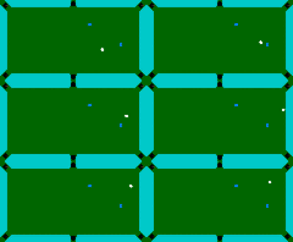
Figure 7. Billiard Ball Environment 1
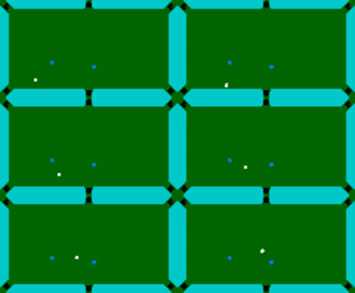
Figure 8. Billiard Ball Environment 2
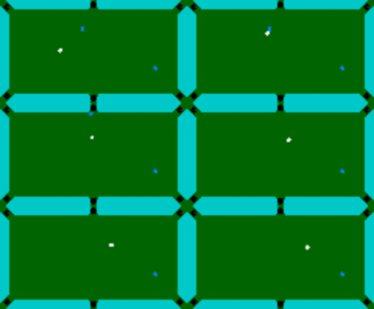
Figure 9. Billiard Ball Environment 3
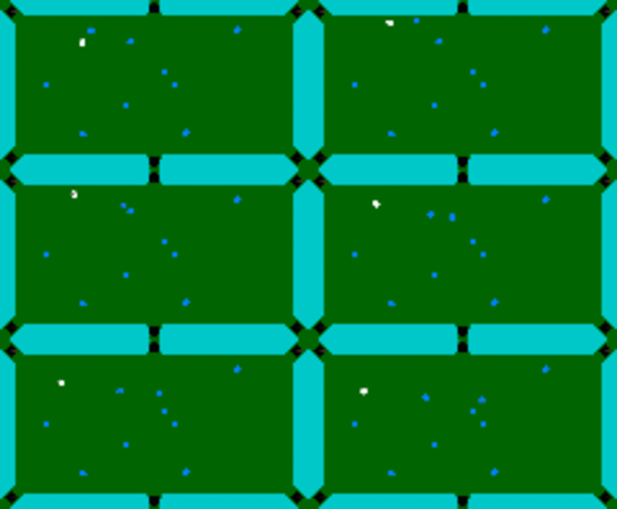
Figure 10. Billiard Ball Environment 4
Next Steps
Since the billiard ball environment is not ready yet we cannot proceed to the planning algorithm. So we plan to finish these two later. After that, we estimate to have some problems with our current method in that the imagined action might not fit the prior very well. So if we directly sample from the prior action, it might fail after long steps. Therefore we need to find some mechanism to ensure our action samples to be stable after enough long steps. It may need us to fit a distribution of the learned action encodings to make the sampling truly work.
Video Presentation
Project presentation
Reference
[1] Thomas Kipf, Elise van der Pol, and Max Welling. “Contrastive learning of structured world models.” 2019.
[2] Robert Kirk, Amy Zhang, Edward Grefenstette, and Tim Rockt ̈aschel. “A survey of generalisation in deep reinforcement learning.” CoRR, abs/2111.09794, 2021.
[3] Thomas M. Moerland, Joost Broekens, Aske Plaat, and Catholijn M. Jonker. “Model-based reinforcement learning: A survey.” 2020.
[4] Haozhi Qi, Xiaolong Wang, Deepak Pathak, Yi Ma, and Jitendra Malik. “Learning long-term visual dynamics with region proposal interaction networks.” CoRR, abs/2008.02265, 2020.
[5] Rishi Veerapaneni, John D. Co-Reyes, Michael Chang, Michael Janner, Chelsea Finn, Jiajun Wu, Joshua B. Tenenbaum, and Sergey Levine. “Entity abstraction in visual model-based reinforcement learning.” CoRR, abs/1910.12827, 2019.
[6] Tianhe Yu, Deirdre Quillen, Zhanpeng He, Ryan Julian, Karol Hausman, Chelsea Finn, and Sergey Levine. “Meta-world: A benchmark and evaluation for multi-task and meta reinforcement learning.” CoRR, abs/1910.10897, 2019.
[7] Klaus Greff, Rapha ̈el Lopez Kaufman, Rishabh Kabra, Nick Watters, Chris Burgess, Daniel Zoran, Loic Matthey, Matthew M. Botvinick, and Alexan-der Lerchner. “Multi-object representation learning with iterative variational inference.” CoRR, abs/1903.00450, 2019.
[8] John Schulman, Filip Wolski, Prafulla Dhariwal, Alec Radford, and Oleg Klimov. “Proximal policy optimization algorithms.” ArXiv, abs/1707.06347, 2017.
[10] “GitHub: packetsss/youtube-projects/pool-game”
[11] “GitHub: DLR-RM/stable-baselines3”