Heterogeneous Multi-agent Reinforcement Learning

In this blog, we are focusing on an algorithm called Embedded Multi-agent Actor–Critic (EMAC) that allows a team of heterogeneous agents to learn decentralized control policies for covering unknown environemnts that includes real-world environmental factors such as turbulence, delayed communication and agent loss, this approch is flexible to dynamic environment elements.

• Overview
• Goal
• Understanding Multi-Agent Actor–Critic (EMAC)
  • Relationships between EMAC and other AC architecture
  • Structures for actor and critic networks
  • How the networks update in EMAC
  • A Broad Look at the Algorithm:
• Environment
• Computation Process
  • Configurations
  • Environment
  • Reward
  • Networks
  • Rollout Storage
• Final Notes on Design
• Challenges
• Next Steps
• Full Implementation
• Final Presentation
• References

Overview

Multi Agent Reinforcement Learning (MARL) studies how multiple agents interact together in an environment to complete specific tasks. The agents can either act cooperatively in which they work together towards the same goal, or act competitively so they accomplish a goal by competing with each other. MARL has incredible achievements in straegy games and it will be the key to the development of sevral emerging technologies such as communications between different autonomous vehicles [3]. MARL systems have been applied to simple tasks that are well-defined with little stochasticity in environment, current methods focus on homogeneous team compositions which allows parameter sharing among actors. Many challenges remain on developing MARL methods that solves more complex and real-word problems with heterogenous team compositions. With such composition, agents will need to leverage their unique abilities and rely on other agents’ specializations to cooperate and find effective policies. Wakilpoor, Ceyer, et al. developed Embedded Multi-agent Actor–Critic (EMAC) which has the ability to interact with the environment dynamically and adjust according to the actions of its team members for more efficient, cooperative behaviors. EMAC allows teams with heterogeneous sensor payload compositions to cover unknown environements. Results show that EMAC outperforms traditional multi-vehicle path planning algorithms as well as independent RL baselines in covering unknown environments [4]. Since the implementation of this algorithm is unpublished, we wanted to compute this algorithm from scratch so that each agent with different observations of the map and with no previous knowledge of the environment can map the entire environment as quickly as possible with their own environment sensors. Therefore, this blog will mainly focus on our computation process.

Goal

• Design a custom environment that mimics the environment in the provided reference paper and that is designed in the gym style
• Build out the EMAC algorithm from the provided algorithm specification as well as integrating it with A2C for parallel rollout as the paper suggests Conduct an ablation study on the performance of CNN versus ANN architectures in the actor and critic roles
• Attempt hyperparameter tuning to deliver SOTA results in the novel HMARL space

Understanding Multi-Agent Actor–Critic (EMAC)

EMAC is fundamentally an actor-critic model that uses independent actor networks with a centralized critic, which allows for a centralized estimate of the value of function with independent execution of policy. EMAC differs from a standard AC architecture in that it supports multi-agent learning with heterogeneous observation sizes. Formally, we can consider each agent capable of providing uniquely sized observations of the state but at the same time using the same actor architecture as we would see in homogeneous cases. With that being said, we thought it would be informative to compare EMAC with other AC archtectures since all expect actor network parity.

Relationships between EMAC and other AC architecture

EMAC VS. Independent Actor-Critic (IAC):

EMAC design aims to address two systemic issues with IAC. First, IAC does not support agent to agent interaction, as the actor and critic network are independent of each other. EMAC addresses this problem by providing a centralized critic that receives the state and current task progress which provides a single value estimate of the state rather than relying on multiple critic networks. Second, IAC does not natively support heterogeneity in agents. This is corrected by providing an embedding layer that takes dynamically scaled observations and converting them to a fixed length feature vector. As we use identical setups for the actor network, it is important that the embedding for each actor provides a similar embedding for a given observation to every other actor. To provide this consistency of representation, we train the embedding layer separately from the actor using the triplet loss which encourages different agents observing the same state to provide similar embeddings. This modification does add additional storage requirements to the project since we now need to store actor sequences for the episode, and the triplet loss requires observations and actions from disparate timesteps.

EMAC VS. Advantage Actor-Critic (A2C):

EMAC suggests the usage of parallel rollout threads with n-agents for stability. We can reconfigure the classic A2C setup with the new EMAC specific modules to support this. Extrinsically, this should improve results with stability and in the meantime allowing for a more rapid training by leveraging a more distributed approach.

A2C doesn’t require much modification for this to work correctly. Instead of storing numerous individual agents in rollout, we store a number of environments which contain multiple agents. As all network updates and environment steps update jointly, we can treat the environment and update rule in the same way that we would treat a single agent programmatically. As previously mentioned, EMAC does have more specific storage requirements, but this can be achieved by increasing the size of the rollout storage. The rollout storage in A2C does not hold the entire trajectory, while a more complete episode trajectory is required in the case of triplet loss, thus we need modifications so that the rollout hold the whole episode.

Structures for actor and critic networks

EMAC does not explicitly require any specific design for the actor and critic network (although it does suggest a fully connected dense layer for the embedding). With this in mind, we propose two possible structures: a classic 3-layer MLP and a 3-layer CNN. Our task is a 2D vision task with various meta-data elements such as the last action, so an MLP with a flatten layer or a 2D convolution block would both be suitable for the actor and critic networks.

How the networks update in EMAC

There are three separate loss functions at play in the EMAC architecture, they are for the actor, critic and embedding layer respectively. The critic is to be updated by mini-batch gradient descent on the MSE of the predicted value of the state versus the reward achieved at that state:

The actor is updated according to an advantage computation with an introduced entropy term to encourage exploration.

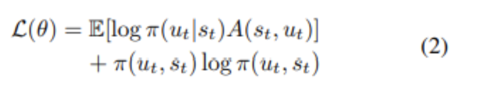
The critic is to be updated by mini-batch gradient descent on the MSE of the predicted value of the state versus the reward achieved at that state:

The embedding layer is updated according to triplet loss which we provide a more thorough explanation of earlier in the writeup. Aside from this triplet loss our implementation is nearly identical, at least in terms of network update, to a standard actor-critic layout.

A Broad Look at the Algorithm:

EMAC adopts a multi-agent actor-critic framework which facilitates centralized policy traning and decentralized policy execution, the key addition to this framework is the embedding network which is a fully connected layer that ingests observations and outputs fixed-length observation encodings, fixed-length encoded observations allows parameter sharing among actors during training, these encoder networks enables heterogeneous sensing capabilities while retaining the training benefits of homogeneous teams.

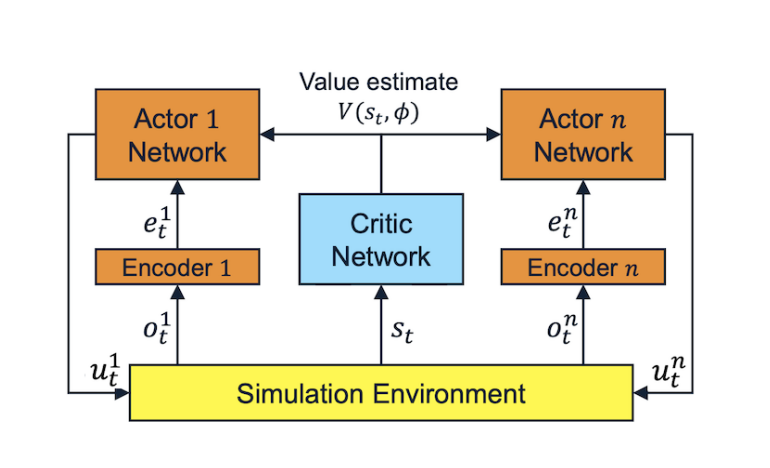
Figure 1. Framework of EMAC

During training, EMAC uses a shared centralized critic to estimate the value function, and each agent encodes observations using a fully connected layer to enable heterogeneous teams. The critic is removed when executing and each agent execute their policies individually, thus, the policies are dependent to the observations.

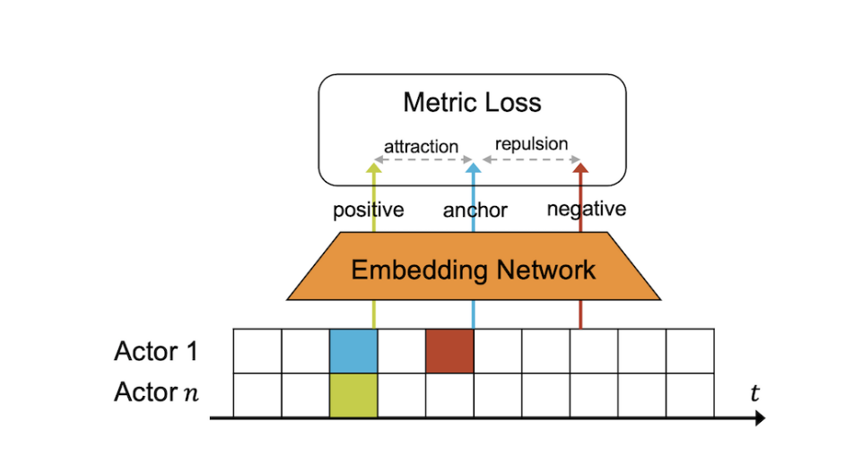
Figure 2. Triplet loss

In order to maintain consistency across the embedding networks, triplet loss is computed to encourage observations coming from the same time but different agents to be pulled together. This time-contrastive loss helps the embedding network to learn embedding representations that explains environmental changes over time. The observation history of an individual agent is the anchor(blue) and it is associated with the positive samples. The green and red represents positive and negative samples respectively, the former is the co-occurring observation history of the agent’s teammate and it comes from different actors at the same time step, while the latter consists of temporal neighbors of the anchor that exceed a minimum time buffer around the anchor which are taken from different times within the same actor sequence. The actor network represents the agent policy function that is shared among heterogeneous agents. The update rule is based on the entire observed trajectory as shown on line 10, we thus set our rollout storage to hold the entire episode as opposed to only a portion of it. Besides that, we also want to provide a brief explanation of what an environment reset looks like in EMAC. Traditionally, RL is based on a repeated exposure to the same environment - in order to encourage generality, however, each environment is randomly generated on a per-episode basis. It is important to consider that heterogeneous multi-agent learning is already difficult to coerce into converging consistently, and that the addition of said randomness can exacerbate this problem, hence the necessity of parallel environments. Aside from these explicit differences, we found that the algorithm is nearly identical to IAC, which is a simple derivation of actor-critic.

Figure 3. Training procedure for EMAC

Environment

Our environment is structurally similar to the grid world but with enough notable differences that it does require its own custom implementation. Every cell in the environment is labeled as being passable, impassable or occupied and a mask is applied to the cells mentioned which indicate whether they have been mapped or not.

Figure 4. Design of the Environment. Each agent is equipped with an environment sensor with a k × k field of view (grey).

In the provided visualization, the agent’s location is represented in a grid marked with ‘a’. We can consider cells with an object in them such as a house or tree as impassible and anywhere else not marked with an ‘a’ as passable. The terrain is also bounded so we only care for the agents to map a specific area, thus, this problem is not an infinite horizon. The goal of the environment is for the agents to view every cell as quickly as possible, on completion the episode is marked as terminal. The action space is not particularly complex either, it provides for a movement in the eight cardinal directions at any given timestep. Notably, there are three marked areas for the agent observation (k, j, and m) which are the sensed terrain, near-field visit history and far-field visit history respectively. For our application we suspect that that far-field visit history is unnecessary and have summarily removed it, but depending on the implementation our readers may find benefit in its inclusion. The sensed region k is simply what is directly observable and the other two regions are what the agent remembers having observed, there is high correlation between the near-field and far-field terrain as they should contain much of the same information. All data that hasn’t been observed yet, likely at the beginning of an episode, is simply padded out with some default value.

Computation Process

Configurations

We based off a modified A2C architecture to support multiple rollout threads and attempt to use that framework to solve the EMAC algorithm. Our hyperparameters and optimizer are both selected directly from the A2C implementation but the specifics of the layer data and initialization should be tuned depending on specific tasks, our parameters are as follows:

COLLISION_PENALTY  = -10
COMPLETION_REWARD  = 100
VISITATION_PENALTY = -10
NUM_STEPS = 100
ENCODER_OUTPUT_DIM = 128
ROLLOUT = 100
GAMMA = 0.99
LR = 7e-4
ENTROPY_LOSS_WEIGHT = 0.01
VALUE_LOSS_WEIGHT = 0.5
GRAD_NORM_MAX = 0.5
NUM_ACTIONS = 8
NUM_AGENTS = 3
ENV_STEPS = 10000

Environment

This is how we initialized our environment:

def __init__(self, size=16, density=0.1, num_agents=3, padding=3):
    self.size = size
    self.padding = padding #if agent is at the edge of grid the environment will pad out impassable terrian so 
    # network has something to read
    self.density = density #how much impassable terrian there is 
    self.observation_space = (padding * 2, padding * 2)
    self.state_space = (size, size)
    self.action_space = 8 # 8 cardinal directions
    self.grid = np.zeros((size, size)).astype(np.uint8)
    block_x = np.random.randint(0, size, size=int((size**2) * density))
    block_y = np.random.randint(0, size, size=int((size**2) * density))
    block_p = np.array(list(zip(block_x, block_y))) #generate random locations for obstacles
    for x, y in block_p:
      self.grid[x, y] = 1
    self.num_agents = num_agents
    self.locations = np.dstack(np.where(self.grid != 1)).squeeze() #generates viable agent placement locations
    self.agents = [ExplorerAgent(self.locations[np.random.choice(self.locations.shape[0])]) for i in range(0, num_agents)]

    self.grid = np.pad(self.grid, pad_width=padding, mode="constant", constant_values=1) # pad out grid
    #padding out grid
    for agent in self.agents:
      agent.x += padding # shift agents over with padding
      agent.y += padding
      self.grid[agent.x, agent.y] = 2 # assign grid location to agent


    self.uncovered_grid = np.zeros((size, size)).astype(np.uint8)
    self.rewards = {agent:0 for agent in self.agents} # Dictionary containing agents and their last step information
    self.step_start_uncovered_ratio = 0.0 
    self.last_move_uncovered_ratio = 0.0
    self.step = 0
    self.max_steps = NUM_STEPS

We provide a solid programmatic approach to constructing our environment leveraging numpy. We’d draw attention to how the grid is being managed to make it as easy as possible to interface with the networks. In particular we pad out the grid so that agents can produce an observation from any point without having to solve indexing issues. We also provide a separate, non-padded grid which holds the cells state, in this case observed or unobserved for the purpose of uncovering based calculations. We also provide some parameters which can be used to conduct generalization experiments including the density of the obstacles and the number of agents the environment should expect. The paper conducts experiments with three heterogenous agents but ideally the environment should work with any team. All representations are handled numerically but could easily be substituted for a richer environmental representation without need of modifying the network architectures - of course by design.

Reward

There are 5 types of rewards:

• 1 = Team-based terminal reward given after completing the grid
• 2 = Team-based progress reward based on the fraction of uncovered cells during timestep
• 3 = Individual discovery reward for cells uncovered
• 4 = Individual visitation penalty if agent didn’t uncover any cells
• 5 = Individual collision penalty if agent collided with terrain or went out of bounds

The rewards are calculated in step_() based on the 5 types of rewards mentioned above, the sum of the reward from each agent will be aggregated later. Besides that, step_() also updates the environment.

  def step_(self, joint_actions):
    done = False
    info = { agent:
              {
                "complete":0, "group_uncover":0, "individual_uncover":0, "visitation_penalty":0, "collision_penalty":0
              } for agent in self.agents
           }

    for agent, action in zip(self.agents, joint_actions):
      action = action.item()
      if not self.is_valid_(agent, action): # Don't move if the action isn't valid
        self.rewards[agent] += COLLISION_PENALTY # Reward 5
        info[agent]["collision_penalty"] = COLLISION_PENALTY
      else: # If the movement is valid that take it
        self.grid[agent.x, agent.y] = 0 # We assume the cell it occupied was passable so just set it back
        agent.move(action)
        self.grid[agent.x, agent.y] = 2 # Update the new cell as containing the agent

      self.set_observed_cells_(agent) # fill in the cells that the agent has observed
      if self.env_done_(): # If the entire grid has been observed then terminate
        done = True
        self.rewards[agent] += COMPLETION_REWARD # Reward 1
        info[agent]["complete"] = COMPLETION_REWARD

      current_uncovered_ratio = self.calc_uncovered_ratio_()
      individual_fraction_uncovered_reward = current_uncovered_ratio - self.last_move_uncovered_ratio
      self.last_move_uncovered_ratio = current_uncovered_ratio

      if individual_fraction_uncovered_reward <= 1e-5:
        self.rewards[agent] += VISITATION_PENALTY # Reward 4
        info[agent]["visitation_penalty"] = VISITATION_PENALTY
      else:
        self.rewards[agent] += individual_fraction_uncovered_reward # Reward 3
        info[agent]["individual_uncover"] = individual_fraction_uncovered_reward

    final_uncovered_ratio = self.calc_uncovered_ratio_() # compute final uncovered reward ratio for agent
    timestep_fraction_uncovered_reward = final_uncovered_ratio - self.step_start_uncovered_ratio
    self.step_start_uncovered_ratio = final_uncovered_ratio

    for agent in self.agents: # update each agents reward
      self.rewards[agent] += timestep_fraction_uncovered_reward # Reward 2
      info[agent]["group_uncover"] = timestep_fraction_uncovered_reward

    self.step += 1 # go to the next step
    obs = self.observe_()
    reward = self.rewards_(info)
    done = np.array([done] * NUM_AGENTS)
    return obs, reward, done

Networks

We firstly set up the encoder which is an embedding layer. Since different observations from different agents might be in various sizes, the embedding layer enables us to take dynamic input of observations and scale it into fixed length vector so they are consistent in size. This step ensures the uniformity of data which is later feed into the actor network.

class Encoder(nn.Module):
  def __init__(self, input_dim, output_dim):
    super(Encoder, self).__init__()

    self.embedding = nn.Linear(input_dim, output_dim)
  def forward(self, obs):
    if len(obs.size()) == 3:
      obs = torch.flatten(obs, start_dim=1)
    else:
      obs = torch.flatten(obs)
    
    x = self.embedding(obs)
    return x 

Critic network is a shared centralized critic to estimate value fuction $V(St,ø)$, critic parameters $ø$ are updated by mini-batch gradient descent. We used Multilayer Perceptron (MLP) that generates a value approximate for the state given the current state and the current observed cells.

class CriticNetwork(nn.Module):
  def __init__(self, state_size, hidden_units=100):
    super(CriticNetwork, self).__init__()
    state_size = np.prod(state_size)

    self.critic = nn.Sequential(
        nn.Linear(state_size, hidden_units),
        nn.ReLU(),
        nn.Linear(hidden_units, hidden_units),
        nn.ReLU(),
        nn.Linear(hidden_units, 1)
    )

  def forward(self, state):
    if len(state.size()) == 3:
      state = torch.flatten(state, start_dim=1)
    else:
      state = torch.flatten(state)

    value = self.critic(state) 
    return value

The CNN critic is an alternate implementation of the critic network which doesnt rely on flattening of the state, but instead relied on the 2-D representation of the state, we anticipated CNN vs MLP will be the same but we wanted to see if there was any performance difference.

class CNNCritic(nn.Module):
  def __init__(self, state_size, hidden_units=100):
    super(CriticNetwork, self).__init__()

    self.critic = nn.Sequential(
        nn.Conv2d(state_size, hidden_units, kernel_size=3, stride=1),
        nn.ReLU(),
        nn.Conv2d(hidden_units, hidden_units*2 kernel_size=3, stride=1),
        nn.ReLU(),
        nn.MaxPool2d(hidden_units*2, hidden_units//2)
        nn.Linear(hidden_units//2, 1) 
    )

  def forward(self, state):
    if len(state.size()) == 3:
      state = torch.flatten(state, start_dim=0)
    else:
      state = state

    value = self.critic(state) 
    return value

Actor network represents the agent policy function, it accepts a fixed-length encoded observation so it’s shareable among heterogenous agents.

class ActorNetwork(nn.Module):
  def __init__(self, input_dim, output_dim, num_actions, hidden_units=100):
    super(ActorNetwork, self).__init__()
    self.encoder = Encoder(input_dim, output_dim) #Encodes network because it's expected to be varibale length
    
    self.actor = nn.Sequential(
        nn.Linear(output_dim, hidden_units),
        nn.ReLU(),
        nn.Linear(hidden_units, hidden_units),
        nn.ReLU(),
        nn.Linear(hidden_units, num_actions)
    )
    self.train()

  def forward(self, obs):
    x = self.encoder(obs)
    logits = self.actor(x)
    return logits #Produce an action by examining the confidence in actions, we want to pick one with highest confidence

Rollout Storage

Traditionally, rollout stores the most recent set of observations and other data in an uncertain setting, so that the next state can be simulated from the current state for the purpose of training. Our implementation still relies on this idea but requires much heavier storage requirements for appropriate updating of the embedding network. We select a rollout size that matches the original implementation while allowing all trajectory data to be stored so that we can use triplet loss. This is equivalent to subsetting the rollout storage depending on what is needed.

Final Notes on Design

There are a couple of other important points in building out the algorithm. We provide three separate loss functions and optimize against three separate network architectures using RMS propagation. This particular selection is preferred over Adam as Adam is targeted to large supervised machine learning tasks where RMS is a more bare-bones implementation of stochastic and mini-batch gradient descent which we feel better fits here. Naturally the parameters for each optimizer will need to be different as the target architectures are different. We recommend providing a bayesian grid search - as the environment is relatively quick to train a robust grid search is feasible and will likely yield the best results. We also recommend providing gradient clipping for both the actor and critic network to prevent overly large updates especially given that HMARL is notoriously unstable. Finally we think that it is best to provide early monitoring for the network to ensure initial convergence in addition to appropriate weight initialization typically done with xavier initialization.

Challenges

One of the major issues for the project was debugging the flow of tensor operations. Because we move so much more data per environment and the number of constituent networks in play is much greater, we found that often a tensor would have an in-place operation performed on it. This would put the tensor in the incorrect state because the gradient wouldn’t record the operation and would later cause problems in backpropagation. In specific, we had originally given each agent a reference to the critic network so that the could fully encapsulate the EMAC algorithm without requiring a secondary object to hold the centralized critic information. This seemed to cause an issue with the state of the tensor and caused us considerable problems in debugging. Our processes involved using the:

torch.autograd.set_detect_anomaly(true)

function to print the underlying C++ stack trace to find which operation was in-place. Unfortunately, detect anomaly only shows a list of potential functions that could have caused the tensor to be in the wrong state and each one needs to be manually debugged to determine if it is causing the problem. One thing that helped solve this was using:

critic_loss.backward(retain_graph=True)
loss.backward(retain_graph=True)

Which allows the loss function to preserve operations that were conducted in the last backwards pass. Eventually it was determined that providing a reference to the critic network as opposed to operating on the network directly caused some internal issue with pytorch and we reconfigured the architecture to reference a secondary object responsible for managing the critic network.

Next Steps

Currently, the embedding layer is not trained because we weren’t able to compute the triplet loss due of the sudden dropout of one of our teammates. Without the triplet loss, we can not backpropogate to update the embedding layer. Therefore, we need to implement triplet loss in our next step so that our EMAC can train the agents properly with an updating embedding layer. After the completion of this algorithm, we would like to run some generlization experiments, such as:

• Use CNN instead of dense layers in our networks to make comparisons
• Create an environment with wind turbulence, agent’s action will change to a neighboring action with probability p
• Create an environment where agents dropout with probability p until the number of agents reached an arbitrary minimum, dropped agents will no longer take actions
• Performing additional studies into team composition and size as our environment is uniquely designed to support it

Full Implementation

https://github.com/JoshuaDuquette2/CS-269-Final

Final Presentation

https://youtu.be/X0TY9Jq-Kec

References

1. Liviu Panait, Sean Luke. “Cooperative Multi-Agent Learning: The State of the Art.” Autonomous Agents and Multi-Agent Systems, vol. 11, no. 3, 2005, pp. 387–434., https://doi.org/10.1007/s10458-005-2631-2.

2. Goyal, Sharma, et al. “CH-MARL: A Multimodal Benchmark for Cooperative, Heterogeneous Multi-Agent Reinforcement Learning.” Robotics Science and Systems Workshop, 2022, https://doi.org/https://doi.org/10.48550/arXiv.2208.13626.

3. Haou, Pierre. “Multi-Agent Reinforcement Learning (Marl) and Cooperative AI.” Medium, Towards Data Science, 8 June 2022, https://towardsdatascience.com/ive-been-thinking-about-multi-agent-reinforcement-learning-marl-and-you-probably-should-be-too-8f1e241606ac.

4. Wakilpoor, Ceyer, et al. “Heterogeneous Multi-Agent Reinforcement Learning for Unknown Environment Mapping.” Artificial Intelligence in Government and Public Sector, 6 Oct. 2020, https://arxiv.org/abs/2010.02663.