Exploring Deep Transformer Q-Networks (DTQN)

In recent years transformers have been vastly used and studied for a variety of supervised learning tasks, especially in the domain of natural language processing (NLP). To utilize their power in capturing long dependencies in sequences, scalability, simplicity and efficiency, transformers have been fused with reinforcement learning tasks. This however till the advert of DTQN was done primarily in an offline RL fashion. Also, previous methods reformulate RL tasks as sequence prediction tasks. DTQN follows the traditional view of Deep Q-learning and can use transformers in an online fashion. We wish to embark upon understanding and dissecting the intricate workings of DTQN in this project.

• Motivation and Introduction
• Video Recording
• Related Work (November 11 update)
  • Deep Q Networks (DQN)
  • Deep Recurrent Q-Learning Networks (DRQN)
  • Deep Transformer Q-Networks (DTQN)
• Comparison with SOTA Transformer-RL method
• Environments
  • CartPole
  • Acrobot
  • LunarLander
• Methodology and Experiments
  • Different loss functions
• Analysis on Experiments
  • Comparing different loss functions
  • Experimenting with LunarLander
  • Experimenting with Acrobot
  • Comparing different network architectures
• Conclusion
• Requirements
• Related Work

Motivation and Introduction

Transformers are powerful models that are capable of learning long sequences. Their self-attention mechanism allows them to learn long dependencies and extract patterns. Given the success of transformers in self-supervised pre-training and fine-tuning to supervised tasks in the natural-language domain, RL practitioners have tried to combine transformers with reinforcement learning concepts [1][2]. Recently in NeurIPS 2022 Workshop a new variant of Deep Q-Network (DQN) was published called Deep Transformer Q-Network (DTQN) [3].

As DTQN is proposed to be highly modular, in this project, we dissect and understand the DTQN model through empirical analysis. We analyse how changing key components and blocks in DTQN affects performance.

Video Recording

Video: Project Overview.

Link To Youtube Video

Related Work (November 11 update)

To understand DTQN we need to understand DQN and DRQN. We train and evaluate on three different models for existing OpenAI Gym environments (CartPole, Acrobot, and LunarLander). The three main models we will be evaluating are:

• Simple DQN Network
• RNN-based DRQN Network
• Transformer-based DTQN Network

Deep Q Networks (DQN)

A DQN fundamentally consists of a mapping table, called the Q-table, which maps a state-action pair to a Q-value. The dimensions of the Q-table are (s,a) where s: state and a: action. The DQN has two main neural networks, the Q-network and Target network. It also consists of a component known an Experience Replay, which interacts with the environment to generate training data. (seen in Fig. 1.)

Figure 1. DQN Architecture

Deep Recurrent Q-Learning Networks (DRQN)

A DRQN is designed by adding a Recurrent Neural Network (RNN) on top of a simple DQN. DQN. The architecture of DRQN augments DQN’s fully connected layer with a LSTM. The last L states are fed into a CNN to get intermediate outputs. These intermediate outputs are then fed to the RNN layer, which is used to predict the Q-value. (seen in Fig. 2.)

Figure 2. DRQN Architecture

Deep Transformer Q-Networks (DTQN)

DTQN uses a transformer decoder structure which incorporates learned position encodings. The model training is done using Q-values generated for each timestep in the agent’s observation history. Specifically, given an agent’s observation history, a DTQN is trained to generate Q-values for each timestep in the history. Each observation in the history is embedded independently, and Q-values are generated for each observation sub-history. Only the last set of Q-values are used to select the next action, but the other Q-values can be utilized for training. (seen inf Fig. 3.)

Figure 3. DTQN Architecture

Comparison with SOTA Transformer-RL method

As suggested by Prof. Bolei Zhou in the mid-term review we do a comparison of DTQN with popular approaches fusing transformers and RL.

Decision Transformer (2021) [1]:

• Offline Reinforcement Learning.
• Agent trained in a supervised fashion.
• Abstracts RL to a sequence learning problem. Allows for drawing upon simplicity and scalability of Transformer architecture, and associates advances in language modeling with RL.
• Does not fit value-functions or policy gradients.
• Rather directly outputs optimal action using a causally masked Transformer.
• Trains an auto-regressive model on reward, previous-state, and actions to predict the next action that should be performed.

Trajectory Transformer (2021) [2]:

• Offline Reinforcement Learning
• Disregards the traditional view of RL problems that utilize Markov property to estimate stationary policies or single-step methods.
• Reformulates this as a traditional sequence learning task.
• Shows flexibility of framework across long-horizon dynamics prediction, imitation-learning, and offline-RL.

DTQN (2022) [3]:

• Online Reinforcement Learning
• Works on POMDP (partially observable Markov decision process) where observations give a noisy or partial state of the world. Using transformers allows for remembering multiple past observations.
• Builds upon previous work on DRQN which uses RNNs that are frail.
• DTQN is modular in its design.

Environments

CartPole

The goal is to balance a pendulum which is placed upright on a cart (attached using an un-actuated joint). The force can be applied from the left or the right direction. link

Acrobot

Two straight pieces are liked together using a joint, with one of the pieces fixed and the other free to move. The goal is to apply torque to the joint so that the tip of the free piece reaches a particular height. link

LunarLander

The goal is the classic rocket trajectory problem. The actions are either engine off or on, which is the only way to control the movement of the rockets. link

Methodology and Experiments

1. Given the novel DTQN, we wish to explore its different components and perform empirical analysis on the changes we make in the network. Specifically, we study the effect of using different loss functions. There are many popular losses such as l2-loss, hinge-loss, etc in the literature. We plug 6 different losses and compare the performance on CartPole (original environment used in the paper).

2. Apart from tweaking the model, we train DTQN with the best loss function on new environments of Acrobot or LunarLander (these environment are not studied in the original paper).

3. We change the architecture of the DTQN to see if a particular network configuration works better. To denote a network architecture by [x,y,z] where x = number of neurons in the first linear layer, y = number of neurons in the second linear layer, z = number of attention heads in multi-head attention. a. First set of experiment deal with changing linear-layer-1 (x) and linear-layer-2 (y) b. In the second set of experiments linear-layer-1 = 64 and linear-layer-2=32 but we change the value of total-number of attention heads (z).

Different loss functions

Mean Squared Error (MSE):

MSE is one of the most common loss functions for supervised learning. In this we take the difference square the difference between the predicted output and actual output. These squared values are then averaged. This is also called L2-norm. MSE is never negative.

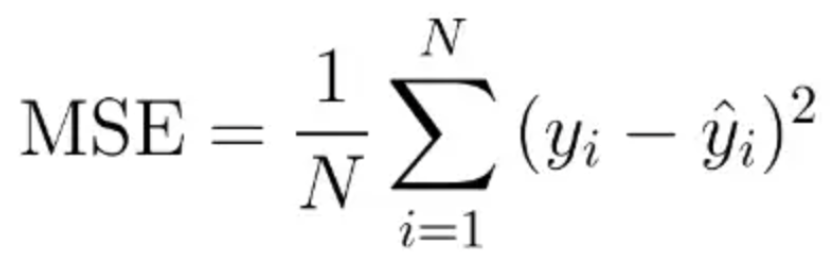
Advantage: There is emphasis on learning outliers as these errors get magnified due to the power of 2. Disadvantage: Given the power function a very big error might bias the learning (for example if there is a very big outlier).

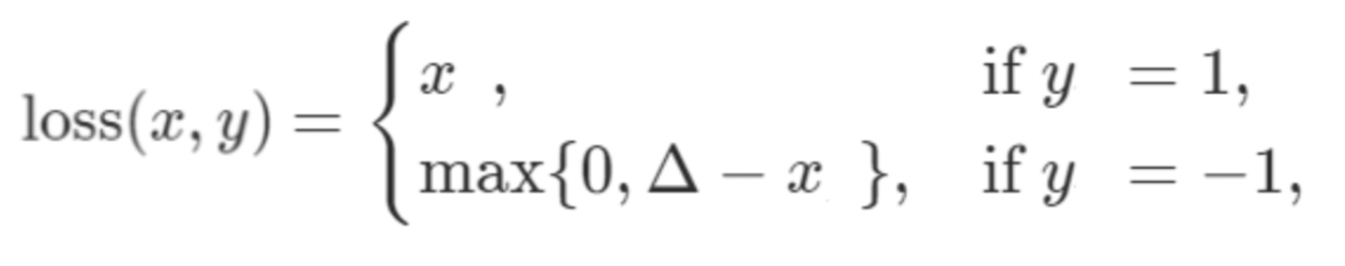
Hinge Embedding Loss:

This loss is used when there is an input x and output y {-1,1}. The formulation penalizes if there is a false prediction of a sign, and promotes predicting the right sign. Here delta is the margin. This loss function is typically very useful for learning non-linear embeddings or for semi-supervised tasks.

L1-norm:

This loss is also called the mean absolute error (MAE). To calculate, we find the absolute error between the predicted value and actual value. These error terms are then averages to get MAE. Similar to MSE this loss is always positive. But this typically has the opposite effect as MSE.

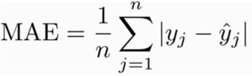
Advantage: Directly opposite to MSE, this loss equally gives importance to each loss, as there is no power function. Outliers do not get special emphasis.

Huber Loss:

This is a piecewise function that finds a balance between MSE and MAE. For loss value less than delta use MSE and for loss value greater use MAE. This enables one to maintain quadratic function near the center for smaller error values because of MSE, and using MAE for large error values allows for more uniform learning.

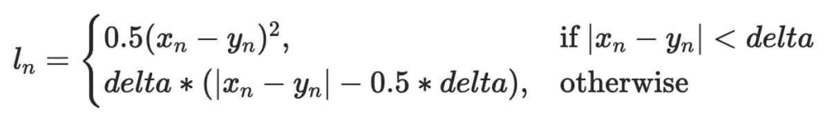
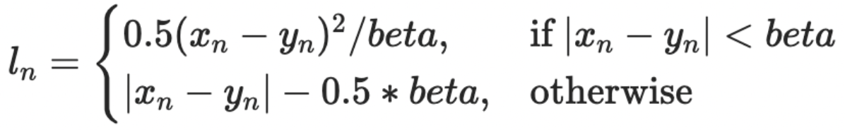
Smooth L1-Loss:

This loss is similar to Huber, with different values of constants for scaling. But the overall effect is similar to huber. This can be considered a mid-way between MSE and MAE.

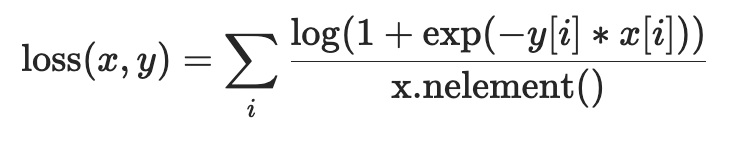
Soft Margine Loss:

Optimize a two-class classification objective logistic loss.

Analysis on Experiments

Comparing different loss functions

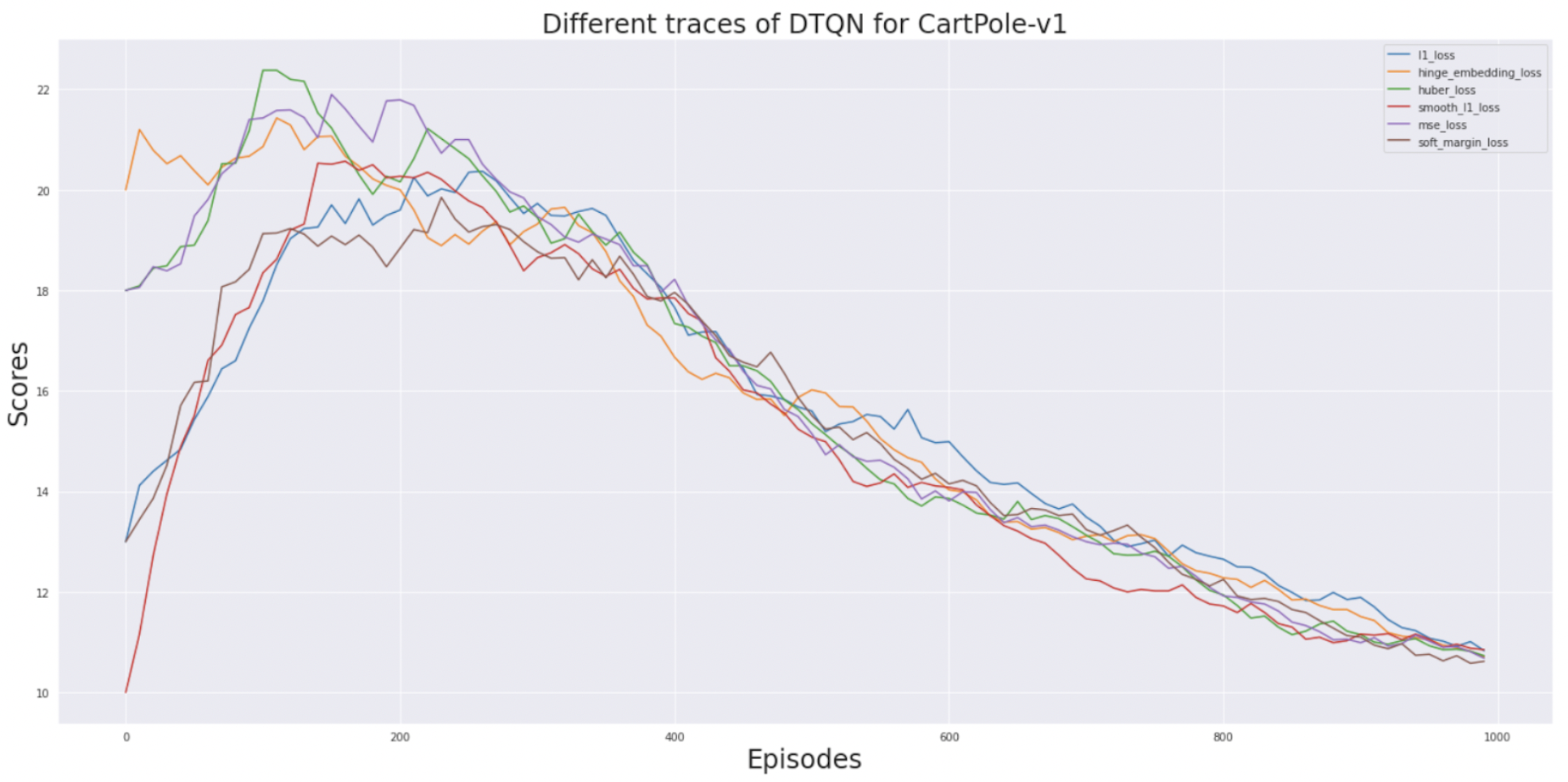
We ran each loss function on CartPole and plot the rewards. L1-loss and MSE are commonly used in the literature for deep reinforcement learning tasks. We wanted to see if huber loss and smooth l1-loss, which are a tradeoff between the two loss functions, perform well for a given reinforcement learning task. But as we see that l1-loss itself is the most stable objective function (blue line in the graph). Apart from showing the most stability it also has the highest reward as compared to other loss plots.

Experimenting with LunarLander

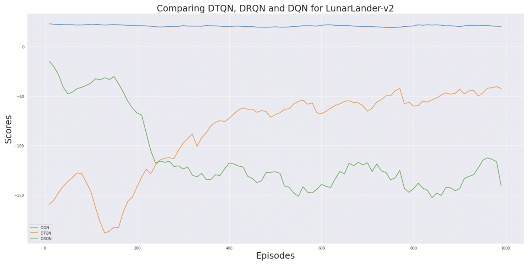We train DQN, DRQN, and DTQN on LunarLander for 1000 epochs (intial learning). Tracking the reward scores of DTQN it can be seen that there is a steady increase as it sees more training epochs. It is way more stable that DRQN, which often oscillate because of instability. DRQN makes use of RNNs that have forget gates which cannot learn dependencies across large temporal relations. The transformer networks in DTQN are more capable. We believe that as train the network for more epochs it will surpass the performace of DQN even. To study this we run LunarLander for larger number of epoch.

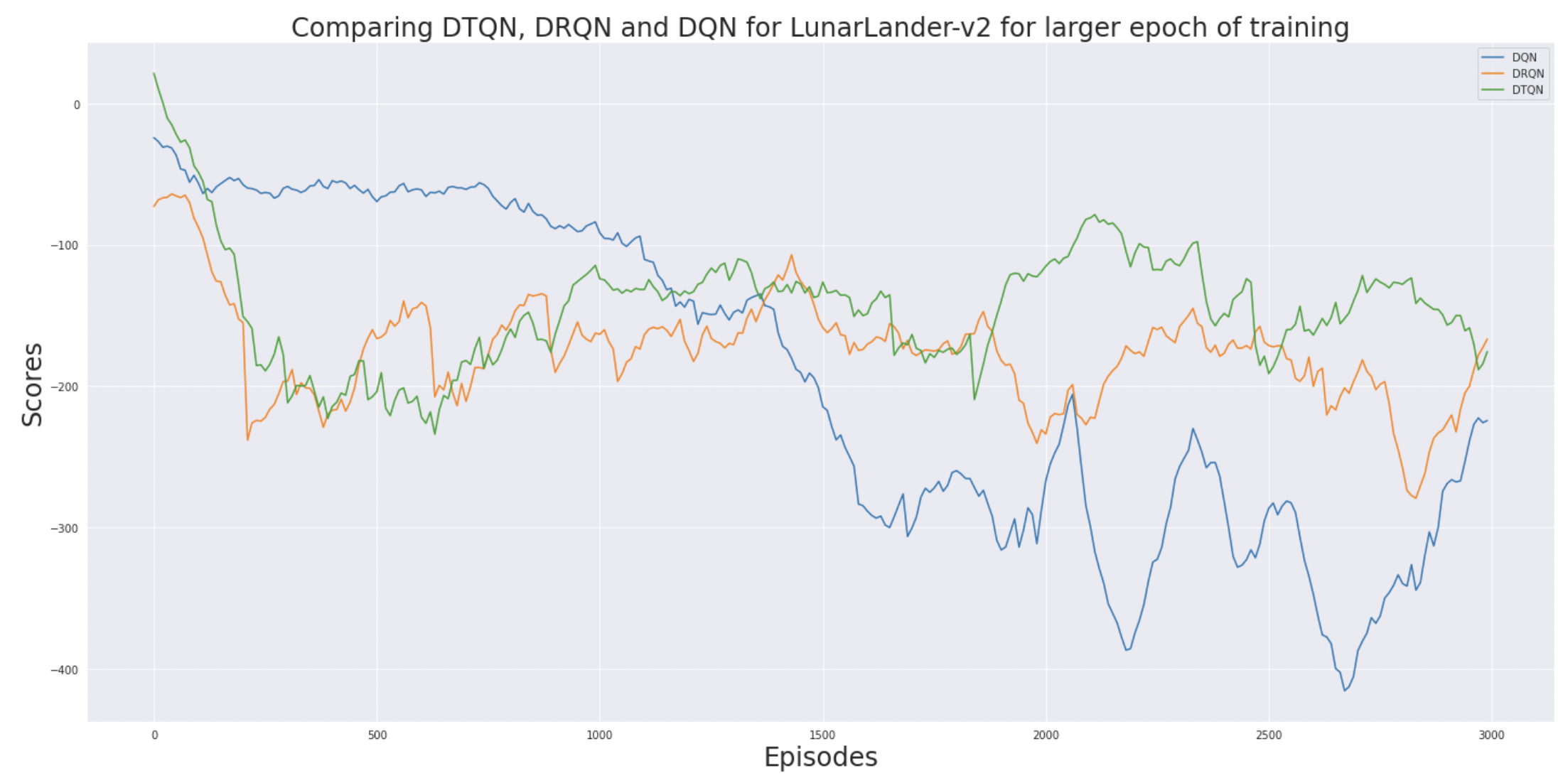Based on our early analysis (mid-term review) we felt that running for a longer duration will change the results. If you see the reward line for DQN it steeply declines we its trained more. Whereas DTQN and DRQN both outperform DQN. Additionally, DRQN is very unstable as compared to DTQN. Finally, DTQN has the highest reward with just a additional epochs of training.

Experimenting with Acrobot

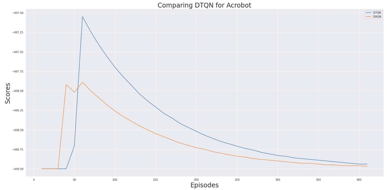We can see that DTQN has be more stable reward output during training as compared to DRQN. This is one of the main objectives of DTQN and this plot confirms the same.

Comparing different network architectures

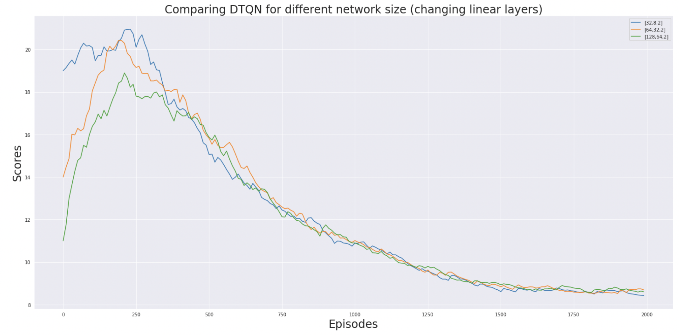We see that changing the size of linear-layers does not have much effect on the reward scores. [64, 32] seems to be the most stable out of the three. All networks nearly perform the same, this maybe because the CartPole is not a complex enough environment to see a difference.

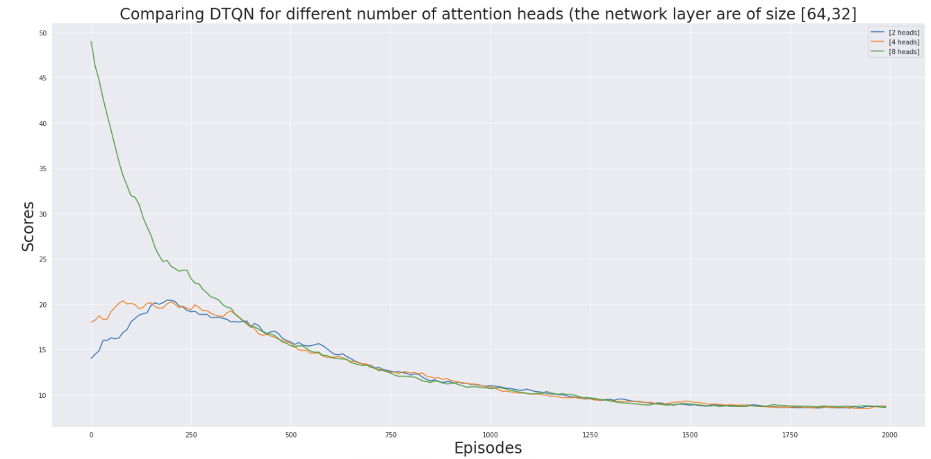Similarly changing attention head does not really have much effect on the performace.

Conclusion

This project primarily focuses on evaluation Transformers in the domain of RL. To verify that Transformers do outperform existing approaches with their modularity, stability and efficiency, we compare 3 different RL architectures namely DQN, DRQN and DTQN. Each model is run in 3 discrete OpenAI Gym environments (CartPole, LunarLander, Acrobot). DTQN was observed to be more stable and obtain better accuracy than DRQN. Further, 6 different loss functions are compared. The L1 loss function was observed to outperform the other 5 loss functions. To test the architecture stability of DTQN, a few architecture variations are proposed and compared. On experimenting, it was concluded that changing the size of the linear layers had nearly no effect on the reward. Further, although all variations performed similarly, the [64,32,2] architecture configuration performed slightly better.

Future work can include extending this work to continuous environments and increasing the complexity of the Transformers used.

Requirements

• OpenAI Gym
• PyTorch
• Python3
• Anaconda Environment
• tensorboardx
• tensorflow

Related Work

1. Lili Chen, Kevin Lu, Aravind Rajeswaran, Kimin Lee, Aditya Grover, Michael Laskin, Pieter Abbeel, Aravind Srinivas, Igor Mordatch. (2021). Decision Transformer: Reinforcement Learning via Sequence Modeling. https://arxiv.org/abs/2106.01345
2. Janner, M., Li, Q., & Levine, S. (2021). Offline Reinforcement Learning as One Big Sequence Modeling Problem. arXiv. https://doi.org/10.48550/arXiv.2106.02039
3. Esslinger, K., Platt, R., & Amato, C. (2022). Deep Transformer Q-Networks for Partially Observable Reinforcement Learning. arXiv. https://doi.org/10.48550/arXiv.2206.01078
4. Boustati, A., Chockler, H., & McNamee, D. C. (2021). Transfer learning with causal counterfactual reasoning in Decision Transformers. arXiv. https://doi.org/10.48550/arXiv.2110.14355
5. Zheng, Q., Zhang, A., & Grover, A. (2022). Online Decision Transformer. arXiv. https://doi.org/10.48550/arXiv.2202.05607
6. Paster, K., McIlraith, S., & Ba, J. (2022). You Can’t Count on Luck: Why Decision Transformers Fail in Stochastic Environments. arXiv. https://doi.org/10.48550/arXiv.2205.15967
7. Wang, K., Zhao, H., Luo, X., Ren, K., Zhang, W., & Li, D. (2022). Bootstrapped Transformer for Offline Reinforcement Learning. arXiv. https://doi.org/10.48550/arXiv.2206.08569
8. Brandfonbrener, D., Bietti, A., Buckman, J., Laroche, R., & Bruna, J. (2022). When does return-conditioned supervised learning work for offline reinforcement learning?. arXiv. https://doi.org/10.48550/arXiv.2206.01079
9. Xu, M., Shen, Y., Zhang, S., Lu, Y., Zhao, D., Tenenbaum, J. B., & Gan, C. (2022). Prompting Decision Transformer for Few-Shot Policy Generalization. arXiv. https://doi.org/10.48550/arXiv.2206.13499
10. Villaflor, A.R., Huang, Z., Pande, S., Dolan, J.M. & Schneider, J.. (2022). Addressing Optimism Bias in Sequence Modeling for Reinforcement Learning. Proceedings of the 39th International Conference on Machine Learning, in Proceedings of Machine Learning Research 162:22270-22283 Available from https://proceedings.mlr.press/v162/villaflor22a.html.
11. Upadhyay, U., Shah, N., Ravikanti, S., & Medhe, M. (2019). Transformer Based Reinforcement Learning For Games. arXiv. https://doi.org/10.48550/arXiv.1912.03918
12. Zhu, Z., Lin, K., Jain, A. K., & Zhou, J. (2020). Transfer Learning in Deep Reinforcement Learning: A Survey. arXiv. https://doi.org/10.48550/arXiv.2009.07888
13. Hausknecht, M., & Stone, P. (2015). Deep Recurrent Q-Learning for Partially Observable MDPs. arXiv. https://doi.org/10.48550/arXiv.1507.06527