Reinforcement Learning for Autonomous Driving in a Realistic Simulated Urban Environment
Investigating the performance of various reinforcement learning strategies for self driving vehicles.
- Introduction
- CARLA Setup
- MetaDrive Environment
- Algorithms
- Methodology
- Results
- Possible Futher Research Directions
- Conclusions
- References
- Appendix
Introduction
Autonomous driving has been a research problem that has been tackled from many different angles. One method often utilized is supervised learning-based computer vision systems where the algorithm is trained using a dataset to identify various objects in the environment, and thus in combination with an algorithmic solution, the vehicle can detect and classify objects in the wild and respond accordingly. Another approach is imitation learning which uses expert (human) examples of driving, and combining that with certain reinforcement learning algorithms so a vehicle can learn to navigate an environment by either completely or mostly copying the behavior of the expert driving examples fed into the system. The third main method is a pure reinforcement learning-based system. Reinforcement learning works by having an agent interact with the environment where beneficial behaviors are rewarded and negative behaviors are penalized, this allows the algorithm to learn how to navigate an environment in a way that maximizes the reward it gets. This has the potential to achieve superhuman performance, but overall is tricky since environment specifics (such as a car shouldn’t cross over the double-yellow line in a roadway) are not hardcoded into the algorithm, the algorithm must learn not to break these various rules. We investigate purely reinforcement learning-based solutions for autonomous driving and learn some insights regarding how well it solves the problem of autonomous driving. We also provide some suggestions how these algorithms could be implemented in an autonomous driving system to provide the best performance.
CARLA Setup
Installing CARLA on a local machine is relatively straightforward. It involves downloading a package from github and running a few scripts to prepare the simulator. However, being able to run the simulations on Google colab would facilitate group work, and running CARLA on colab is difficult. Just running the colab example that CARLA provides causes warning popups to appear, and requires the installation of cloudflare and TurboVNC viewer. Furthermore, it was found that Google Colab no longer allows remote desktop connection to their instances, which is an essential part needed to run CARLA.
These additional requirements made us choose to work with MetaDrive instead. MetaDrive offers a much simpler API that is more compatible with google colab.
MetaDrive Environment
Using MetaDrive in colab is very simple, requiring only a few pip install commands and dependency imports.
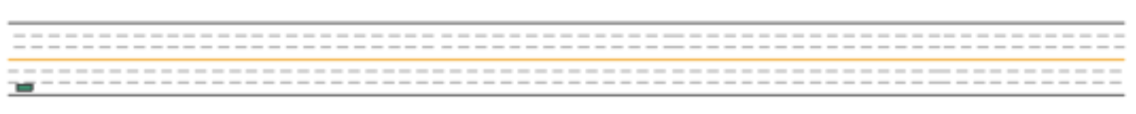
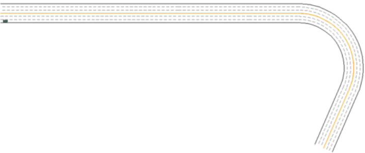
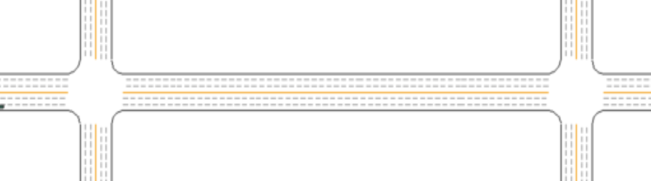
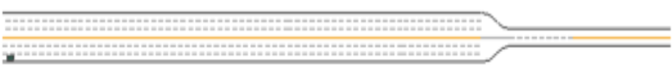
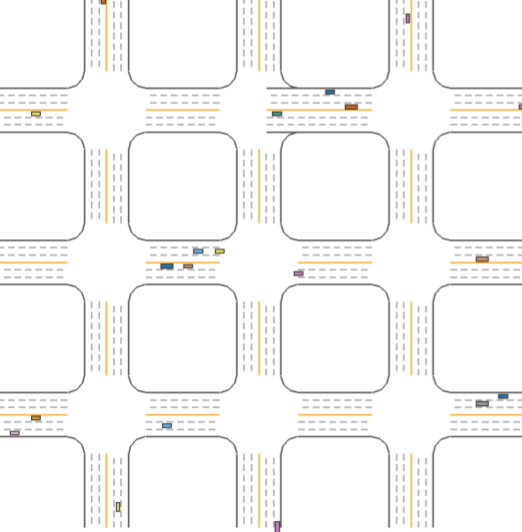
To build the environment that our models would train in, we used MetaDrive’s map customization feature which allows us to specify a string to determine the blocks each map is composed of. We chose to run our tests on 5 different environments: a basic straight road, a road with two intersections, a road that goes from more lanes to fewer lanes, a straight road that ends with a curve, and a 3x3 grid of intersections (similar to the default environment in CARLA).
MetaDrive uses a combination of distance traveled, speed, and termination state as the metric to calculate the episodic reward when training a model. During model evaluation, the run terminates if the agent car crosses the yellow line divider, collides with another car on the road, or hits the road barrier.
Straight Road Environment
Curved Road Environment
Two Intersections Environment
Narrowing Road Environment
3x3 Grid Environment
Algorithms
DQN
Deep Q-Networks (DQN) is a reinforcement learning algorithm that uses a deep neural network to approximate the action-value function, Q(s, a) in order to select optimal actions to take in a given state. This network is trained using a variant of the Q-learning algorithm, which uses experience replay and a target network to stabilize the learning process.
During training, DQN collects experiences in the form of state-action-reward-next tuples, which are then used to improve the neural network. One key attribute of DQN is that it uses an epsilon-greedy strategy to approach the exploration-exploitation tradeoff.
To update the network, a target value is calculated:
\[y = r + \gamma * max_a Q'(s',a)\]Where \(r\) is the reward, \(\gamma\) is the discount factor, \(Q'(s', a)\) is the predicted state-action value of the next state.
Then, the loss is calculated using \(L = (y - Q(s,a))^2\), and the network’s weights are updated via \(w = w + alpha * gradient(L)\)
PPO
Proximal Policy Optimization (PPO) is a type of reinforcement learning algorithm that uses a neural network to approximate the agent’s policy. PPO uses an iterative process called policy optimization. The first step is where the agent collects batches of experiences by interacting with the environment and following the existing policy. These experiences feed into the neural network, which then improves the accuracy of the policy. This process repeats until the policy has reached an optimum.
Each time the policy is updated, it is always close to the previous one, this ensures the learning process is stable and does not change too much in any one step, which could lead to poor performance.
The objective function (used to measure the quality of the policy and update network weights) is calculated using \(L = min(r(s,a) * A(s,a), clip(r(s,a), 1-\epsilon, 1+\epsilon) * A(s,a))\) where \(r(s, a)\) is the probability ratio, \(A(s, a)\) is the advantage, and \(\epsilon\) is the gradient clipping parameter.
Then, the policy loss \(L_{pi}\) is used to update the weights of the policy network:
\[L_{pi} = -L\] \[\theta = \theta + \alpha * gradient(L_{pi})\]Where \(\alpha\) is the learning rate, \(gradient(L_{pi})\) is the gradient of the policy loss with respect to the weights \(\theta\).
The value loss is calculated as the MSE of the predicted and expected (target) values via \(L_v = (V_{target}(s) - V(s))^2\). The value loss is then used to update the weights \(w\) of the value network using \(w = w + \alpha * gradient(L_v)\)
REINFORCE
REINFORCE is a reinforcement learning algorithm that uses Monte Carlo methods to estimate the agent’s policy and value function. REINFORCE uses the total rewards that the agent receives over a number of steps to update the policy.
The process of REINFORCE is to: (a) collect a batch of experiences by interacting with the environment by following the current policy, (b) use those experiences to estimate the value of each state and the expected return of each action, (c) update the policy based on the estimated values and returns, and (d) use the updated policy to collect more experiences.
The state-value function \(V(s)\) is updated using the Monte Carlo return (sum of the discounted rewards for a given episode) via \(V(s) = V(s) + \alpha * (G - V(s))\), where \(G\) is the monte carlo return, \(\alpha\) is the learning rate, and \(V(s)\) is the state-value function.
TD3
TD3 is an extension of the Deep Deterministic Policy Gradient (DDPG) algorithm. It uses a neural network to approximate a policy and value function. The extension from DDPG is that TD3 uses two separate networks to approximate the policy and value functions, rather than a single network. These two networks are known as the “actor” and “critic”. The actor network chooses the action that the agent will take at each step, while the critic is used to estimate the value of each state.
To improve the stability of the learning process, TD3 also employs a technique called “delayed policy updates”, where the policy is only updated every few steps (rather than at every one step). This prevents the policy from being changed too quickly.
The value function \(Q(s, a)\) is updated using \(Q(s, a) = Q(s, a) + \alpha * (y - Q(s, a))\), where \(y\) is the expected future return, or the target value, which is calculated with \(y = r + \gamma * V(s`)\). Here r is the reward, gamma is the discount, and \(s'\) is the next state. The value of the next state is obtained by maximizing over actions taken in the next state.
Methodology
We use the 5 metadrive environments described above to run a set of baseline experiments on using the 4 reinforcement learning algorithms discussed above: DQN, PPO, REINFORCE, and TD3. From this, we derive some insights and then run further experiments as extensions that provide additional useful insights.
Results
Experiments’ Quantitative Results
Default hyperparameters used for experiments listed below in appendix.
Initial Experiments
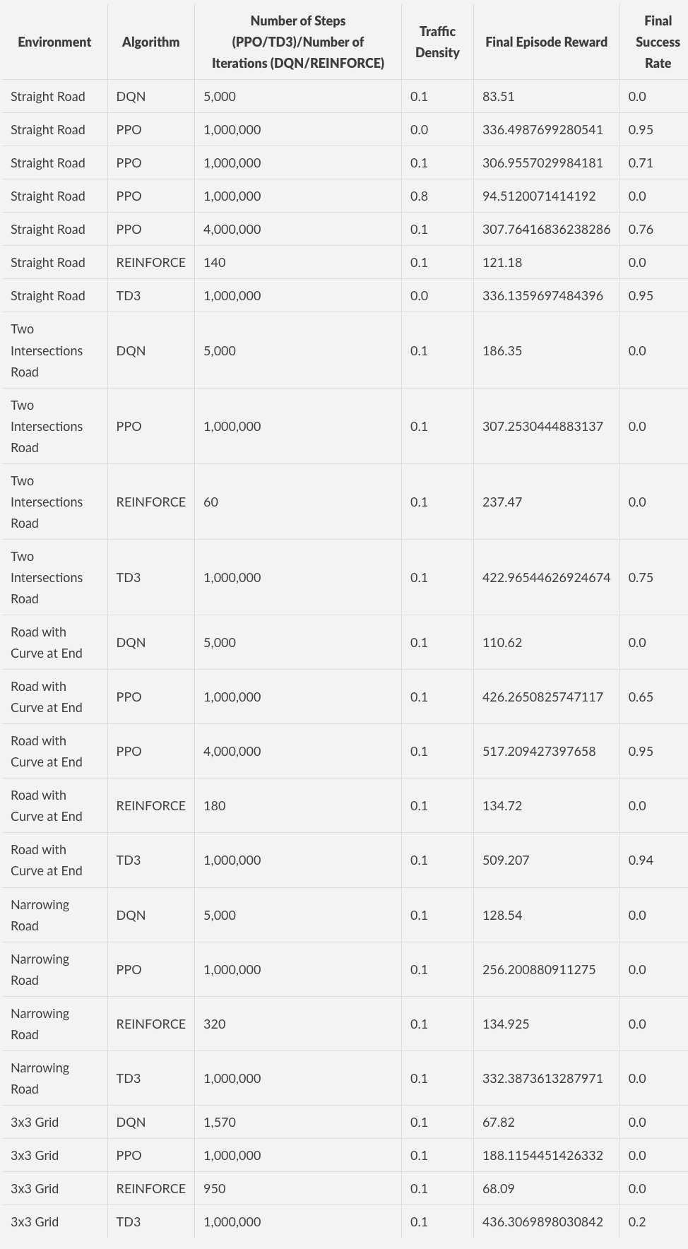
For PPO and TD3, we set the max-steps by default to 1,000,000 unless marked otherwise.
In these experiments, success rate refers to the number of episodes where the agent reaches the destination over the number of episodes that were tested. Episode reward is a more arbitrary reward measure that simply allows us to see if the algorithm is growing in performance. As such success rate is correlated with episode reward, but the correlation varies based on the specific environment involved since an easier environment can be solved (giving 1.0 success rate) with less of an episode reward usually. Traffic density is the number of vehicles per 10 meters per traffic lane.
Overall, it was found that DQN and REINFORCE had greater difficulty solving the environments compared to PPO and TD3. In particular, even when removing the cap on interactions for our implementation of REINFORCE in the road with two intersections environment, it was found that after a given amount of iterations, the episode reward improvement stopped improving and leveled off at around 237.
Unsurprisingly, when controlling the environment, and only adjusting traffic density, as seen with our experiment on the basic straight road, the problem difficulty increases with the amount of traffic on the road. Though this does not give the entire story, as shown with a later experiment in the further experiments section.
When comparing the performance of PPO and TD3 across environments, they give largely similar performance when controlling the number of steps used, however a small edge can be given to TD3, particularly when in more complicated environments and it also typically gives a better success rate when compared to PPO. This may well be attributed to the fact that TD3 is an actor-critic method while PPO is a policy gradient method, and actor-critic methods are typically more sample efficient compared to policy gradient methods. We did notice, however, during execution that the TD3 episode reward tended to jump around more while the increase in PPO episode reward was more linear.
Finally, we found that simpler environments were easier to solve compared to more difficult environments, specifically when it came to success rate. The order of difficulty (from least to greatest) in our experiments is the following: basic straight road, road with curve at end, road with two intersections, road that narrows, and 3x3 grid environment. This ordering is based on the final achieved episode reward and success rate.
Further Experiments
We conducted a series of experiments using the extra heavily trained version of the PPO agent in the curved road environment, this agent was trained using 4,000,000 steps rather than just 1,000,000. It was trained with a traffic density value of 0.1. This result led to a 0.95 success rate in the curved road environment.
First it was tested to see how the improved PPO agent would perform in the same environment (road with curve), except with no traffic. Interestingly, it had lower episode reward (345.970) compared to the episode reward it got in its training environment which had some traffic (517.209). When looking at the animation of vehicle driving in both traffic scenarios, it almost seems the agent learned to follow the vehicles in the scene to correctly navigate the curve and not hit the double-yellow line (which results in a fail), thus when in an environment with no other vehicles, the agent usually ends up eventually hitting the double-yellow line.
We then test to see how the improved PPO agent would perform in the two intersections environment. Interestingly here, when there was traffic, it performed quite poorly compared to the baseline, with an episodic reward of 159.129. However, when the two intersections environment had no traffic, it performed pretty well, nearly reaching the end of the route and achieving an episodic reward of 412.666, which is not significantly far off from the baseline reward of 517.209.
It was also seen that in the 3x3 grid environment, DQN and REINFORCE struggled significantly where the episodic reward would stop improving past the low scores of (around 68 for both). We had to stop the training in both instances since there was no improvement past around 68 for many iterations.
Another interesting observation is that the performance of the 4,000,000 step straight road PPO agent on the straight road environment was not much better than that of the respective 1,000,000 step straight road PPO agent. This seems to show that increasing the step count for training a PPO agent can only go far in improving the agent’s performance in an environment and that there are diminishing improvements after a certain point.
Possible Futher Research Directions
It would be interesting in the future to see how these algorithms perform in training an agent on a single large environment that involves all the various features from each of the environments we made. It would also be interesting to see if better performance for a more complete reinforcement learning-based autonomous driving solution would use multiple agents, with a classifier that would detect the environment a vehicle is in, and then have the vehicle driven by the agent that performs best in that given environment.
Conclusions
Overall, the experiments we conducted gave interesting insights into how reinforcement learning algorithms perform on the problem of autonomous driving. We found that simpler techniques such as DQN and REINFORCE had a lot more trouble learning a driving environment compared to more advanced algorithms such as PPO or TD3. Unsurprisingly, greater performance was achieved through allotting greater training time (through increasing the maximum number of steps). We found that agents had a hard time generalizing to other environments and other traffic conditions. It seems like if one were to train a reinforcement learning agent for autonomous driving, they would need to test it in a very systematic manner on every single possible scenario a vehicle may encounter (including every form of traffic condition) before attempting to deploy it in an actual vehicle. Finally we found that the various algorithms we tested had increasing amounts of difficulty of solving more complicated environments. Overall, we find that the algorithms we tested in their current form are insufficient in solving the problem of autonomous driving, and other methods or tweaks would have to be employed, on top of having significantly more computational resources, to come anywhere near having an autonomous driving system that is at least somewhat safe.
References
CARLA Environment
[Dosovitskiy, et al.] “CARLA: An Open Urban Driving Simulator” https://arxiv.org/pdf/1711.03938.pdf
[Li, et al.] “MetaDrive: Composing Diverse Driving Scenarios for Generalizable Reinforcement Learning” https://arxiv.org/pdf/2109.12674.pdf
Appendix
Default Hyperparameters Used for Experiments
DQN
Max Episode Length: 1000
Max Number of Iterations: 5000
Evaluation Interval: 50
Evaluate Number of Episodes: 5
Learning Rate: 0.0001
Clip-Norm: 10
Memory Size: 1000000
Learn Start: 5000
Eps: 0.1
Target Update Frequency: 5000
Learn Frequency: 16
Batch Size: 256
PPO
Number of Parallel Environments: 10
Seed: 0
Number of Steps: 2000
Learning Rate: 0.00005
Lambda: 0.95
Number of Epochs per Training Iteration: 10
REINFORCE
Training Batch Size: 2000
Normalize Advantages: True
Max Episode Length: 200
Max Iteration: 5000
Evaluation Interval: 10
Evaluation Number of Episodes: 10
Learning Rate: 0.001
Clip-Norm: 10
TD3
Initial Random Policy Steps: 1000
Batch Size: 64
Exploratory Noise: 0.2
Learning Rate: 0.00005
Discount Factor: 0.99
Target Network Update Rate: 0.005
Target Policy Noise: 0.2
Target Policy Noise Clip Range: 0.5
Delayed Policy Update Frequency: 2